Phase Equilibria Calculation of CO 2 System at Given Volume, Temperature, and Moles in CO 2

(1)

Phase Equilibria Calculation of

CO

₂

−

H

₂

O

System at Given Volume, Temperature, and Moles

in

CO

₂

Sequestration

Tereza Jindrov´a, and Jiˇr´ı Mikyˇska

Abstract—The paper deals with the investigation of multi-phase equilibrium of CO2−H2Osystem at constant volume, temperature and moles (the so-called V T-flash), which is motivated by topical problem of CO2 sequestration. Study-ing CO2 −H2O mixture under natural geological conditions (pressures typically below 50MPa and temperatures typically 298–383K) for different system composition, two-phase and three-phase states were observed. Recently, we have developed a fast and robust algorithm for constant-volume two-phase split calculation, which is based on the direct minimization of the total Helmholtz free energy of the mixture with respect to the mole- and volume-balance constraints. The algorithm uses modified Newton-Raphson minimization method. To initialize the algorithm, an initial guess is constructed using the results of constant-volume stability testing. In this work, we extend the results for CO2 −H2O system and propose a fast and robust algorithm for three-phase equilibrium computation at constant volume, temperature and moles. The performance of the proposed strategy is shown on several examples of two- and three-phase equilibrium calculations of CO2−H2O mixture under various conditions. Finally, we discuss the fact that the V T-approach seems more natural than the widely used classical formulation at constant pressure, temperature and moles (the so-calledP T-flash), especially when using pressure-explicit equations of state.

Index Terms—phase equilibrium, constant volume flash,CO2 sequestration, Helmholtz free energy minimization, Newton-Raphson method, modified Cholesky factorization.

I. INTRODUCTION

S

TUDYING CO2−H2Osystem phase behaviour is mo-tivated byCO2 sequestration, which is from an ecology point of view a possibility of protection against the green-house effect by capturing emissions ofCO2at the source and storing them into deep geological repositories (technology

CCS- Carbon Capture and Storage) or salt-water reservoirs. For such operations, it is essential to fully understand the thermodynamics of the processes in the subsurface and to have a model which describes the behaviour ofCO2correctly under wide range of natural geological conditions.

Manuscript received December 24, 2013; revised July 21, 2014. The work was supported by the projects LH12064 Computational Methods in Thermodynamics of Hydrocarbon Mixtures of the Ministry of Education of the Czech Republic, P105/11/1507 Development of Computer Models of CO2 Sequestration in the Subsurface of the Czech Science Foundation, by the research direction project MSM6840770010 Applied Mathematics in Technical and Physical Sciences of the Ministry of Education of the Czech Republic, and by the project SGS11/161/OHK4/3T/14 Advanced Supercomputing Methods for Implementation of Mathematical Models of the Student Grant Agency of the Czech Technical University in Prague.

T. Jindrov´a and J. Mikyˇska are with the Department of Mathematics, Faculty of Nuclear Sciences and Physical Engineering, Czech Technical University in Prague, Trojanova 13, 120 00 Prague 2, Czech Republic, e-mail: [email protected] .

InjectingCO2into a reservoir, it may dissolve in the water or it can mix and the CO2−H2O mixture can split into two or more phases. Let us consider a closed system of total volumeV containing aCO2−H2Omixture with mole numbers Nw, Nc at temperature T. First, we are interested

to find out whether the system is under given conditions in single-phase or splits into two phases. This is the problem of single-phase stability at constant volume, temperature and moles (the so-calledV T-stability). In case of phase-splitting we want to establish volumes of both phases, mole numbers of each component in both phases, and consequently the equilibrium pressure of the system from the equation of state. This is the problem of two-phase split calculation at constant volume, temperature and moles (the so-calledV T -flash). In our previous work [5], [6], [7], these problems were formulated and the algorithms were proposed and tested on many examples.

The formulation of phase stability investigation and phase-equilibria computation at constant volume, temperature and moles is alternative to the traditional formulation at constant pressure, temperature and chemical composition, which has been used in many applications [1], [2], [3], [4], [8], [9]. Despite the well-known fact that there is the possibility of using alternative variables, in most applicationsP T-stability andP T-flash have been used to solve the phase stability and phase-equilibria computation and the algorithms fully based on V T variables started to be developed only recently [5], [6], [7].

To demonstrate the shortcomings of the traditional vari-ables, let us consider pure CO2 at temperature T = 280 K and saturation pressure Psat(T) corresponding to the

tem-perature T = 280 K. Using traditional P T variables, one cannot decide whether the system occurs in vapor or liquid state, or as a mixture of both, because all two-phase states and both saturated gas and saturated liquid occur at the same pressure, which is equal to the saturation pressure

Psat(T), temperature and moles. Therefore, P T-stability

and P T-flash cannot distinguish between these states, but

V T-stability and V T-flash can, because these states have different volumes. This example shows that theP T-stability andP T-flash problems are not well posed since the volume of the system is not uniquely determined by specifying the pressure, temperature and moles. On the other hand, if volume, temperature and moles are specified, the equilibrium pressure is given uniquely by the equation of state. The non-uniqueness of volume at specified pressure, temperature and moles for the pure substances at saturation pressure has been discussed in [5], [6], [7]. In this work, we present a non-trivial example of a binary mixture of CO2−H2O in

IAENG International Journal of Applied Mathematics, 45:3, IJAM_45_3_03

(2)

three phases, which exhibits the same behaviour as the pure substances at saturation pressure.

In [5], we have developed and successfully tested a nu-merical algorithm for constant-volume two-phase split cal-culation which is based on the constrained minimization of the total Helmholtz free energy of the mixture. The algorithm uses the Newton-Raphson method with line-search and modified Cholesky decomposition of the Hessian matrix to produce a sequence of states with decreasing values of the total Helmholtz free energy. Using of the Newton-Raphson method ensures fast convergence around the solution. Fur-thermore, as the method guarantees decreasing in the total Helmholtz free energy of the system in every iteration, it always converges to a state corresponding to at least a local minimum of the energy. To initialize the algorithm, we use the results of the constant-volume stability algorithm which has been developed in [7]. In this work, we extend these re-sults to three phases forCO2−H2Osystem, which provides us a better understanding of the thermodynamic behaviour of CO2mixtures under geologic carbon storage conditions, and present an algorithm for three-phase equilibrium computation at constant volume, temperature and moles. The performance of the proposed strategy is shown on several examples of two- and three-phase equilibrium calculations ofCO2−H2O mixture under various conditions.

The paper is structured in the following way. In sec-tion 2, we formulate the V T-flash problem and derive the equilibrium conditions for binary mixture of CO2−H2O using the Helmholtz free energy. In section 3, we describe a new computational algorithm for three-phase equilibrium calculation at constant volume, temperature, and moles. In section 4, we summarize key steps of the algorithm and propose a general strategy for the constant-volume phase-split calculation of CO2 −H2O system. In section 5, we present numerical results showing the performance of the algorithm onCO2−H2Omixture under different conditions. In section 6, we discuss the results, especially, we point out advantages of using V T-variables instead of traditional

P T-variables, and draw some conclusions. In the Appendix, we provide details of the Cubic-Plus-Association equation of state [12], [13] that was used in the work.

II. PHASEEQUILIBRIUMCONDITIONS FORCO2−H2O SYSTEM

Consider a closed system containing a binary mixture of water(H2O)and carbon dioxide(CO2)with mole numbers

NwandNc occupying total volumeV at temperatureT. Let

us assume that the mixture occurs in anN-phase state, where

N = 2 or N = 3, and denote the volumes of each phase

Vαand the mole numbers of each component in each phase

Nα,w andNα,c, where α= 1, . . . , N. We are interested in

deriving conditions ofN-phase equilibrium in the mixture. Let us denote by x0 and xα vectors with components

Nw, Nc, V and Nα,w, Nα,c, Vα, where α = 1, . . . , N,

re-spectively. Then, for the single-phase CO2−H2O system, the Helmholtz free energy is given by

AI =A(x0, T) =−P V + X

i=w,c

Niµi, (1)

where P =P(x0, T) is the pressure given by a pressure-explicit equation of state, andµi=µi(x0, T)is the chemical

TABLE I LIST OFNOTATION

Symbol meaning

A Helmholtz free energy

bi covolume parameter of the Peng-Robinson EOS

c molar concentration

δX−Y binary interaction coefficient between componentsX andY

i, j component indices;wfor water,cfor carbon dioxide

k iteration index

kB Boltzmann constant

µα,i chemical potential of thei-th component in phaseα

Mw,i molar weight of thei-th component

Nα,i total mole number of thei-th component in phaseα

N number of phases

ωi accentric factor of thei-th component

P pressure

Pi,crit critical pressure of thei-th component

R universal gas constant

T absolute temperature

Ti,crit critical temperature of thei-th component

V total volume of the system

Vα volume of phaseα

zi overall mole fraction of thei-th component

potential of thei-th component in the mixture. For the N -phase system, the total Helmholtz free energy reads as

AN =

N

X

α=1

A(xα, T). (2)

An equilibrium state of theN-phase system is such a state for which the increase in the total Helmholtz free energy with respect to an energy reference state

∆A =

N

X

α=1

A(xα, T)−Aref, (3)

where the energy reference stateAref can be chosen for ex-ample as a single-phase state or an(N−1)-phase equilibrium state, is minimal among all states satisfying the following constraints expressing the volume balance and mole balance

N

X

α=1

Vα=V, (4)

N

X

α=1

Nα,i=Ni, i=w, c. (5)

Using the Lagrange multiplier method, we derive the system of necessary conditions of the phase equilibrium

P(x1, T) =· · ·=P(xN, T), (6)

µi(x1, T) =· · ·=µi(xN, T), i=w, c. (7)

Let us denote byPeq the equilibrium pressure, which is the common value of pressures in each phase, and by µeq_i the chemical potential of thei-th component in the equilibrium, which is the common value of chemical potentials of thei-th component in each phase.

IAENG International Journal of Applied Mathematics, 45:3, IJAM_45_3_03

(3)

III. NUMERICALALGORITHM FORCOMPUTATION OF

THREE-PHASEEQUILIBRIUM FORCO2−H2OSYSTEM

We derive a numerical algorithm for testing three-phase equilibrium of CO2 − H2O system at constant volume, temperature and moles based on minimization of the total Helmholtz free energy of the three-phase system (3) which is subject to the volume and mole balance constraints (4) and (5). In all these equations, we setN = 3and we still denote by xα a vector with components Nα,w, Nα,c, Vα, where

α= 1, . . . , N. In general, the numerical procedure is based on transferring ann-dimensional problem of minimization of a twice-continuously differentiable objective function subject to a set oftlinear equality constraints into an unconstrained minimization problem with the same objective function, but a lower dimensionn−t.

The constraint equations (4) and (5) for N = 3 can be written in the matrix form asAx=b,or





1 0 0 1 0 0 1 0 0 0 1 0 0 1 0 0 1 0 0 0 1 0 0 1 0 0 1





| {z }

A





x1

x2

x3 



| {z } x

= 



N1

N2

V





| {z } b

, (8)

where A ∈ R3×9 is the matrix formed by 3 blocks of the

identity matrices in R3_, _x_∈_R9 _{is the vector of unknowns,} which is given as

x= (N1,w, N1,c, V1, N2,w, N2,c, V2, N3,w, N3,c, V3)>

and b ∈ R3 is the vector of right hand side. As the matrix A has the full rank, the optimization problem with

9 unknowns and 3 linearly independent linear constraints can be transformed into an unconstrained problem with 6 variables. The reduction in dimensionality can be described in terms of two subspaces Y and Z, where Y is the 3-dimensional subspace of R9 _{spanned by the rows of matrix}

A and Z is the 6-dimensional subspace of R9 of vectors

orthogonal to the rows of matrix_A. The representation ofY is not unique and it can be chosen for example as Y =AT_.

AsY andZ define complementary subspaces

R9=Y ⊕ Z, (9)

every 9-dimensional vector x can be uniquely written as a combination of vectors fromY andZ as

x=YxY+ZxZ, (10)

where Y and Z denote matrices from R9×3 and R9×6,

respectively, whose columns represent bases of subspacesY andZ, and the3-dimensional vectorxY is called the

range-space part of x, and the 6-dimensional vector xZ is called the null-space part ofx.

The solutionx∗ of the constrained optimization problem, given by

x∗=Yx∗Y+Zx∗Z,

is feasible, whence

Ax∗=A(YxY∗ +Zx∗Z) =b.

From the definition of subspaceZ it follows thatAZ = 0,

therefore

AYx∗Y=b.

From the definition of subspace Y it can be seen that the matrix _AY is non-singular, and thus the vector x∗_Y is uniquely determined by the previous equation. Similarly, any feasible vectorx must have the same range-space part, which means xY = x∗Y, and on the contrary, any vector

with range-space component x∗_Y satisfies the constraints of the optimization problem. Hence, the constraints uniquely determine the range-space partx∗_Y of the solution, and only the 6-dimensional part x∗_Z remains unknown. This way the expected reduction in dimensionality to6 is performed.

To represent the null-space Z, the LQ-factorization of matrix A is used [10]. Let Q ∈ R9×9 be an orthonormal

matrix such that

AQ= L 0, (11)

whereL∈ R3×3 is a non-singular lower triangular matrix.

From (11) one can see that the matrix _Ycan be chosen as the first 3 columns of matrix _Q and the matrix _Z can be chosen as the remaining6 columns of _Q, i.e.

Q= Y Z. (12)

As the matrix of constraintsA ∈R3×9 can be written as

A = I3 I3 I3 ,

then the matricesYandZmay be chosen as

Y= √1

3A

T ₌_√1

3 



I3

I3 

, Z = 1 √ 3





I3 I3

−I3 0 0 −I3



 (13)

For solving the constrained optimization problem we use an iterative algorithm in which a feasible initial guessx(0)

is given and the algorithm generates a sequence of feasible iteratesx(k). In every iteration, the solution x(k) is approx-imated as

x(k+1)=x(k)+λkd(k), (14) whereλk _∈ _{(0; 1i} _{is the step size in the} _k_{-th iteration and}

d(k)_{is the direction vector in the}_k_{-th iteration. We assume} thatx(k)_{is feasible and the feasibility of}_x(k+1)_{is required,} so the direction vectord(k) _{must be necessarily orthogonal} to the rows ofA, i.e.

Ad(k)= 0, (15)

which can be equivalently written as

d(k)=Zd(Zk), (16)

for some 6-dimensional vectord(_Zk). It can be seen that the search directiond(k)_{is a}_{9-dimensional vector constructed to} lie in the6-dimensional subspaceZ. The columns of matrix

Z, which form an orthogonal basis ofZ, are given by (13),

so it remains to determine the vectord(_Zk) ∈R6_{. This way} the constrained minimization problem is transferred to an unconstrained problem in a lower dimension.

To find the vector d(_Zk), we use the modified Newton-Raphson method which is based on the quadratic approxima-tion of funcapproxima-tion∆Aaround the pointx(k). Let us denote by

g(x)∈R9the gradient of the function∆Awhich is obtained

IAENG International Journal of Applied Mathematics, 45:3, IJAM_45_3_03

(4)

by differentiating the∆Awith respect to its variables, i.e.

g(x) =∇(∆A)>=                  

µw(x1, T)

µc(x1, T) −P(x1, T)

µw(x2, T)

µc(x2, T) −P(x2, T)

µw(x3, T)

µc(x3, T) −P(x3, T)

                  . (17)

Further, let us denote by H(x) ∈R9×9 the Hessian of the

function ∆A which is obtained by differentiating the ∆A

twice with respect to its variables in a block-diagonal form with3 diagonal blocks given in the following form

H(x) =∇2∆A=

  H1 H2 H3  ,

Hα(x) =

            

Bα Cα

Cα> Dα

             , (18)

whereα∈ {1,2,3} and

Bα∈R2×2, Bαij =

∂µi

∂Nα,j

(xα, T)

Cα∈R2, Cαj =−

∂P ∂Nα,j

(xα, T),

Dα∈R1, Dα=−

∂P ∂Vα

(xα, T),

wherei, j∈ {w, c}

Approximating the function ∆A using the Taylor expan-sion around the point x(k) _{up to the quadratic terms, the} search directiond(k)₌

Zd(Zk) can be found as a solution of

the following minimization problem

min

d(k)∈R9

Ad(k)₌₀

∆A(x(k)+d(k)) = min d(_Zk)∈R6

∆A(x(k)+Zd(Zk))≈

≈ min d(_Zk)∈R6

∆A(x(k)) +g(x(k))>_Z d(_Zk)+

+1 2(Zd

(k)

Z ) >

H(x(k))Zd(Zk). (19)

Define a quadratic functionΦas

Φ(dZ) =g(x(k))>ZdZ+

1 2d

>

ZZ>H(x(k))ZdZ,

then the vector d(_Zk) is the argument of its minimum. The functionΦhas a stationary point if and only if there is ad(_Zk)

for which the gradient ofΦvanishes, i.e.

∇Φ(d(_Zk)) = 0. (20)

The stationary point d(_Zk) is a solution of the following system of equations

HZ(x(k))d(Zk)=−gZ(x(k)), (21)

where HZ(x(k)) ∈ R6×6 and gZ(x(k)) ∈ R6 are the

restrictions of the Hessian matrix and of the gradient vector to the subspaceZ defined as

HZ(x(k)) =Z>H(x(k))Z (22)

and

gZ(x(k)) =Z>g(x(k)). (23)

Combining (13), (17), and (18), it follows from (23) that

gZ(x(k)) =

1 √ 2           

µw(x1, T)−µw(x2, T)

µc(x1, T)−µc(x2, T) −P(x1, T) +P(x2, T)

µw(x1, T)−µw(x3, T)

µc(x1, T)−µc(x3, T) −P(x1, T) +P(x3, T)

           , (24)

and from (22) that the restricted Hessian matrix can be found in the following form

HZ(x(k)) =

1 2

H2Z H1

H1 H3Z

,

HαZ(x(k)) =

             e

Bα Ceα

e

Cα> _Deα

             , (25)

whereα∈ {2,3},H1∈R3×3 is given by (18) and

e

Bα∈R2×2, _Ceα∈R2, _Deα∈R1, e

Bαij =

∂µi

∂N1,j

(x1, T) +

∂µi

∂Nα,j

(xα, T),

e

Cαj =−

∂P ∂N1,j

(x1, T)−

∂P ∂Nα,j

(xα, T)

e

Dα=−

∂P ∂V1

(x1, T)−

∂P ∂Vα

(xα, T),

wherei, j∈ {w, c} The gradient vector in (17) depends on the values of chemical potentials which can be determined up to an arbitrary constant. Unlike in (17), the restricted gradient given by (24) is a function of differences of the chemical potentials between two states whose values can be evaluated uniquely using the equation of state.

If d(_Zk) solves the system of the equations (21) and the matrix HZ is positive definite, then the search direction d(_Zk) is a descent direction. If the matrix of the projected Hessian is not positive definite, then either the quadratic approximation of the function is not bounded from below, or a single minimum does not exist. In this case, it is necessary to modify the directiond(_Zk). If the matrixHZ is indefinite,

IAENG International Journal of Applied Mathematics, 45:3, IJAM_45_3_03

(5)

then the vector d(_Zk) is found as a solution of a modified system of equations

d

HZ(x(k))d(Zk)=−gZ(x(k)), (26)

whered_HZ(x(k))is a positive definite matrix obtained by the modified Cholesky decomposition of the matrix_HZ(x(k)_{). In} this algorithm the usual Cholesky factorization is performed to decompose matrix HZ(x(k))as

HZ(x(k)) =LL>,

where L is a lower triangular matrix. If a negative

ele-ment appears on the diagonal of L during the Cholesky

factorization, a suitable value is added to this element to ensure its positivity in the final decomposition. This way we obtain the Cholesky factorization of a positive definite matrixdHZ(x(k)), which is used instead of matrix HZ(x(k)) in (26) to determine the direction d(_Zk) in the Raphson method. Due to this modification of the Newton-Raphson method, the obtained direction is a descent direc-tion. Therefore, for a sufficiently small step size λk _> ₀_,

the decrease of ∆A can be guaranteed. In this work, the line-search technique is used to find the step sizeλk. First, we set λk = 1 and test if ∆A(x(k)+d(k)) < ∆A(x(k)). If this condition is satisfied, we set x(k+1) =x(k)+d(k). If not, we halve the value of λk _{unless the condition}

∆A(x(k)₊_λk_d(k)₎ _< _∆_A₍_x(k)₎ _{is satisfied and then set}

x(k+1) ₌ _x(k)₊_λk_d(k)_{. Now, a single iteration of the} Newton-Raphson method is completed.

The iterations are stopped when either the maximal num-ber of iterations is achieved (500), or when a stopping criterion is satisfied and the required accuracy is achieved. In this work the stopping criterion is given by

kd(k)k2:= 

 9 X

j=1

d(_jk) 2





1 2

≤10−7. (27)

IV. ALGORITHM OF THEMODIFIEDNEWTONMETHOD FORCONSTANT-VOLUMETHREE-PHASEFLASH OF

CO2−H2OSYSTEM

Now, we summarize the key steps of the algorithm.

Step 1 LetNw, Nc,V andT >0be given. Set the number

of iterations k = 0. Get an initial feasible solution

x(0)_∈_R9 _{from the}_{V T}_{-stability algorithm [7]}

x(0)= 

            

N1,w

N1,c

V1

N2,w

N2,c

V2

N3,w

N3,c

V3 

            

. (28)

Step 2 Assemble the Hessian matrix HZ(x(k)) and the

gradient vectorgZ(x(k))of∆Ain thek-th iteration

projected to the subspaceZ using (25) and (24).

Step 3 Compute the projected step directiond(_Zk)∈R6and the feasible direction d(k)_∈_R9 _by

HZ(x(k))dZ(k)=−gZ(x

(k)₎_, ₍₂₉₎

d(k)=_Zd(_Zk). (30)

If the matrix HZ(x(k))is not positive definite, find

the vector d(_Zk) by solving a modified system of equations

d

HZ(x(k))d(Zk)=−gZ(x(k)), (31)

wheredHZ(x(k))is a positive definite matrix obtained from the modified Cholesky decomposition of matrix

HZ(x(k)).

Step 4 Determine the step length λk > 0 for the k-th iteration satisfying

∆A(x(k)+λkd(k))<∆A(x(k)). (32) First, set the step length to λk _{= 1} _{and test if the}

condition (32) holds. If not, use the bisection method to find a value ofλk _{satisfying (32).}

Step 5 Update the approximation as

x(k+1)=x(k)+λkd(k). (33)

Step 6 Test the convergence using (27). If needed, increase

kby1and go to Step 2. If not needed, the algorithm ends up with the solutionx(k+1).

Note that the constant-volume stability algorithm from [7] is used to test whether a single phase is stable or not at given conditions. If the mixture is unstable, theV T-stability provides an initial guess - the concentrations of a trial phase, which, if taken in a sufficiently small amount from the initial phase, lead to a two-phase system with lower value of the Helmholtz free energyA than the hypothetical single-phase state. From this, a criterion of stability at constant volume, temperature, and moles can be derived (see [7] for details).

General Strategy for Phase Equilibrium Computation of

CO2−H2OSystem

Using the Gibbs phase rule [8], the maximal number of phases for the binary system ofCO2−H2OisN = 3and the system can exist in single-, two- and three-phase states. The proposed general strategy for phase-equilibrium testing is based on repeated constant-volume stability testing and constant-volume phase-split calculation and can be summa-rized in the following steps:

Step 1 Set the number of phasesN = 1 and perform the constant-volume single-phase stability using the al-gorithm, which is provided in [7]. If the single-phase state is stable, calculate the equilibrium pressure from the equation of state and the procedure ends.

Step 2 If the single phase is unstable, an initial two-phase split is provided from the phase-stability algorithm and the constant-volume two-phase flash algorithm is performed using the method described in [5].

Step 3 Perform the phase-stability algorithm on one of the two equilibrium phases. If it is unstable, an initial guess for the three-phase split calculation is pro-vided.

Step 4 Perform the constant-volume three-phase flash cal-culation to establish composition, densities and amounts of the phases using the algorithm described above.

IAENG International Journal of Applied Mathematics, 45:3, IJAM_45_3_03

(6)

TABLE II

PARAMETERS OF THE PHYSICAL PART OF THE

CUBIC-PLUS-ASSOCIATION EQUATION OF STATE FOR THEH2OAND

CO2MIXTURE(THE NOTATION IS EXPLAINED IN THEAPPENDIX).

Component Ti,crit[K] Pi,crit[MPa] ωi[-] Mw,i[g·mol−1]

H2O 647.29 22.09 0.3440 18.02

CO2 304.14 7.375 0.2390 44.0

V. RESULTS

Studying a binary mixture ofCO2−H2Ounder different conditions, we have tested the proposed algorithm in several examples of general phase-stability testing and phase-split calculation both at constant volume, temperature and moles of CO2 − H2O system. In all simulations we perform isothermal compression of a CO2 − H2O mixture of a given chemical composition zw, zc in a closed cell, where

zw=Nw/N, zc=Nc/N andN=Nw+Nc. Changing the

overall concentrationcat a given temperatureT, we provide the results of the constant-volume two- and three-phase flash calculations for the CO2−H2O mixture at temperature T

and molar concentrations ci = czi. For the CO2 −H2O

system, we use the Cubic-Plus-Association (CPA) equation of state [12], [13]. Parameters for the physical part used are presented in Table II. Details for the equation of state can be found in the Appendix.

Two-Phase Equilibrium of theCO2−H2OSystem

First, we investigate phase equilibrium for a binary mix-ture of water (H2O) and carbon dioxide (CO2) with mole fractionszH2Oranging from0.1to1.0andzCO2 = 1−zH2O

at temperature T = 308.15 K. For this temperature, the binary interaction coefficient is δH2O−CO2 = 0.09850 and

the cross association factor used in the CPA equation of state issCO2 = 0.025936802. Note thatδH2O−CO2 andsCO2 are

strongly dependent on temperature. For T = 308.15 K and mole fractions of water zH2O ranging from 0.1 to 1.0, the

mixture splits in all cases into two phases except from very low overall molar concentrationsc.

Changing the mole fraction of water zH2O from 0.1 to

0.9, the mixture behaviour does not change very much. In all cases it can be seen that the mutual solubility of CO2 and water is limited. Saturations (volume fractions) of both phases as functions of the overall molar concentration c

are presented for three different mole fractions zH2O (0.1,

0.5 and 0.9) in Figure 1. Mole fractions of both water and carbon dioxide components in both phases as functions of the overall molar concentrationcare presented for the same three values of mole fractionszH2O in Figure 2. In Figure 3, mass

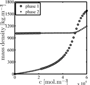
densities of both phases as functions of the overall molar concentrationcare presented forzH2O= 0.9. Note that while

compressing the mixture, its composition in both phases and mass densities of the phases almost do not vary, only slight variations of volume fractions in both phases can be seen. The equilibrium pressure as a function of the overall molar concentration c is presented for mole fraction zH2O = 0.9

in Figure 4 illustrating a steady increase of the equilibrium pressure during compression.

In all cases, quadratic convergence of the Newton-Raphson method has been observed. Thus, numerical errors can be estimated from the size of increment in the last few iterations.

(a)zH2O= 0.1

(b)zH2O= 0.5

[image:6.595.45.304.97.135.2]

(c) zH2O= 0.9

Fig. 1. Saturation of both phases as a function of the overall molar concentrationcfor the binary mixture ofCO2−H2Owith three different values ofzH2OatT = 308.15K.

Using the Euclidean norm, the estimated error is approxi-mately10−14_.

Three-Phase Equilibrium of theCO2−H2OSystem

Now, we investigate phase equilibrium for a binary mixture of water (H2O) and carbon dioxide (CO2) with low mole fractions zH2O ranging from 0.003 to 0.008

IAENG International Journal of Applied Mathematics, 45:3, IJAM_45_3_03

(7)

(a)zH2O= 0.1

(b)zH2O= 0.5

[image:7.595.47.295.45.501.2]

(c)zH2O= 0.9

[image:7.595.337.513.49.237.2]

Fig. 2. Mole fractions of both components in each phase as functions of the overall molar concentrationcfor the binary mixture ofCO2−H2O with three different values ofzH2OatT = 308.15K.

Fig. 3. Mass densities of both phases as a function of the overall molar concentrationcfor the binary mixture ofCO2−H2OwithzH2O= 0.9

atT = 308.15K.

Fig. 4. Equilibrium pressure as a function of the overall molar concen-tration cfor the binary mixture of CO2−H2O with zH2O = 0.9 at

T= 308.15K.

and zCO2 = 1−zH2O at temperature T = 298.15 K.

For this temperature, the binary interaction coefficient is

δH2O−CO2 = 0.078795and the cross association factor used

in the CPA equation of state is sCO2= 0.021141. For

T = 298.15 K and very low mole fractions of water zH2O

ranging from0.003 to0.008, the mixture splits in all cases into two or three phases except from very low overall molar concentrationsc.

Changing the mole fraction of water zH2O from 0.003

to 0.008 and compressing the mixture at temperature

T = 298.15 K, the mixture occurs in two-phase from the lowest molar concentrations up to approximately 9000 mol.m−3_{, then becomes three-phase, while at} mo-lar concentrations higher than 14000 mol.m−3 _{the mixture} becomes two-phase again. Finally, from the molar con-centrations approximately18500 mol.m−3, 23500 mol.m−3 and 29000 mol.m−3, the mixture with zH2O = 0.003,

zH2O= 0.005 and zH2O = 0.008, respectively, becomes

single-phase (see Figure 5, 6 or 7).

In Figure 5, mass densities of each phase as functions of the overall molar concentration c are presented for three values of zH2O, i.e. 0.003; 0.005 and 0.008. Note that in

case ofzH2O= 0.008 while at lower molar concentrationsc

the two-phase region corresponds to a gas-liquid two-phase region, at high molar concentrations c we can observe a second phase area corresponding to a liquid-liquid two-phase region as can be seen from the values of mass densities of the phases (see Figure 5(c)).

Mole fractions of water and carbon dioxide components in each phase as functions of the overall molar concentrationc

are presented for the same three values ofzH2O in Figure 6

in which the limited mutual solubility ofCO2and water can be seen. Saturations (volume fractions) of each phase and also equilibrium pressures as functions of the overall molar concentration c look similar for different values of zH2O,

so we present them forzH2O= 0.003 in Figure 7 and 8. In

Figure 8, the equilibrium pressure as a function of the overall molar concentrationcis presented illustrating a steady rise of the equilibrium pressure during the compression in two-phase area, followed by the constant value of pressure within the

IAENG International Journal of Applied Mathematics, 45:3, IJAM_45_3_03

[image:7.595.84.259.548.713.2]

(8)

three-phase area (for molar concentrations between approx-imately9000mol.m−3 _and₁₄₀₀₀ _mol.m−3_{), demonstrating} the similar behaviour as pure components, and the substantial increase at molar concentrations higher than14000mol.m−3 when the gas phase is depleted. Notice again that as the pressure is constant during the compression in the three-phase region, the mass densities of each three-phase and the composition of each phase remain constant as well.

Numerical errors are comparable to those from the two-phase examples.

VI. DISCUSSION ANDCONCLUSION

To draw some conclusion from the results, it can be seen from Figure 3 that the mass densities of both phases intersect at molar density approximately50000 mol.m−3 _{and switch,} i.e. the heavier phase, which is rich in water, becomes the lighter one and the lighter phase, which is rich in CO2, becomes the heavier one. The pressure corresponding to this molar concentration is approximately40.86 MPa. Similarly, when consider theCO2−H2Osystem withzH2O= 0.008,

the mass densities of both phases intersect in the two-phase region at molar density approximately24000mol.m−3 and switch (see Figure 5(c)). The pressure corresponding to this molar concentration is approximately 37.83 MPa. The switching of phases is an important evidence for CO2 sequestration because if the CO2 −H2O mixture is com-pressed at the level for which the mass densities of both phases intersect and switch (i.e. for molar concentrations higher than 50000 mol.m−3 _{in case of the} _CO

2 −H2O mixture from Figure 3 and for molar concentrations higher than24000mol.m−3_{in case of the}_CO2_−H2O_{mixture from} Figure 5(c)), then the phase rich inCO2becomes heavier and goes down in the reservoir. Consequently, the phase rich in water becomes lighter and goes up, so that another amount of CO2 can be dissolved into it.

As explained in the Introduction, specification of pressure, temperature and moles may not determine uniquely the equilibrium state of the system. In our previous work [5], we have observed this issue in pure substances at saturation pressure in two phases. In this work, the behaviour similar to that of pure components has been observed in case of CO2−H2Osystem in three phases, proving that there exist mixtures more complex than the trivial ones which cannot be fully described using theP T variables. In the plot illustrating pressure as a function of the overall molar concentration (see Figure 8), we can observe the constant plateau within the three-phase area like in the case of pure CO2 within the two-phase region. All these three-phase states occur at the same pressure, temperature and moles, therefore, they are indistinguishable in terms of the P T variables, but can be distinguished using the V T variables because the volumes are different in these states. The results of the algorithm testing provide an important evidence that the P T andV T

variables are definitely not equivalent and that by specifying the pressure, temperature and moles the equilibrium state cannot be uniquely determined in pure component as well as in more complex systems.

To conclude, in this work we have extended the results of the previous work, in which we have dealt with the problem of single-phase stability and two-phase split calculation in a multicomponent mixture in a closed cell, both at constant

(a)zH2O= 0.003

(b)zH2O= 0.005

(c)zH2O= 0.008

Fig. 5. Mass densities of each phase as a function of the overall molar concentrationcfor the binary mixture ofCO2−H2Owith three different values ofzH2OatT = 298.15K.

volume, temperature and moles (the so-called V T-stability andV T-flash), to the constant-volume three-phase equilib-rium computation for the binary mixture of CO2−H2O under geologic sequestration conditions. The performance of the algorithm is shown on several examples of two- and three-phase equilibrium computations of the mixture which is described using the Cubic-Plus-Association equation of state. In future work, the algorithm will be generalized and

IAENG International Journal of Applied Mathematics, 45:3, IJAM_45_3_03

[image:8.595.323.502.45.619.2]

(9)

(a)zH2O= 0.003

(b)zH2O= 0.005

[image:9.595.42.300.52.524.2]

(c)zH2O= 0.008

Fig. 6. Mole fractions of both components in each phase as functions of the overall molar concentrationcfor the binary mixture ofCO2−H2O with three different values ofzH2OatT = 298.15K.

the behaviour of mixtures in three and more phases is to be investigated to draw some general conclusions.

APPENDIX

EQUATION OFSTATE

In this work we use use for the mixture of water (H2O) and carbon dioxide (CO2) the Cubic-Plus-Association (CPA) equation of state [12], [13].

This equation is based on the Peng-Robinson equation of state [11] to describe the physical interactions and the termodynamic perturbation theory to describe the bonding of water molecules. We assume that each water molecule has four association sites of two types (mark them α and

β), so each type has two sites. We assume the same for each molecule of carbon dioxide, whose association sites can be marked as α0 and β0. Let χα and χβ be the mole

[image:9.595.336.512.52.227.2]

fractions of water not bonded at site α andβ, respectively,

Fig. 7. Saturation of each phase as a function of the overall molar concentrationcfor the binary mixture ofCO2−H2OwithzH2O= 0.003 atT= 298.15K.

Fig. 8. Equilibrium pressure as a function of the overall molar concentration

cfor the binary mixture ofCO2−H2Owith zH2O = 0.003 atT =

298.15K.

and letχ_α0 andχ_β0 be the mole fractions of carbon dioxide not bonded at siteα0 andβ0, respectively. Assuming neither cross association nor self association between carbon dioxide molecules, and symmetric cross association between the two sites of different type of water and carbon dioxide, we obtain the following simplified expressions for the symmetric association model

χα=χβ =χw=

1

1 + 2Nw

V χw∆αβ+ 2 Nc

V χc∆αβ

0,

χ_α0 =χ

β0 =χc=

1

1 + 2Nw

V χc∆αβ

0.

In these equations the association strength between molecules of water is given by

∆αβ=gκαβ[exp(αβ/kBT−1)],

wherekB is the Boltzmann constant,καβ and αβ are the

bonding volume and energy parameters of water, respec-tively, and g is the contact value of the radial distribution function of hard-sphere mixture that can be approximated

IAENG International Journal of Applied Mathematics, 45:3, IJAM_45_3_03

[image:9.595.338.513.280.467.2]

(10)

TABLE III

PARAMETERS OF THECPAEQUATION OF STATE FOR THEH2OANDCO2

MIXTURE(THE NOTATION IS EXPLAINED IN THEAPPENDIX).

Symbol Units Value

καβ _[m3_mol−1_] ₁_.₈₀₁₅₀₆_·₁₀−6

αβ_/k

B [K] 1738.393603

a0

w [J·m−3·mol−2] 0.096273

c1 [-] 1.755732

c2 [-] 0.003518

c3 [-] -0.274636

as g=g(η)≈1−0.5η

(1−η)3, where η = B

4V and B is the

pa-rameter from the Peng-Robinson equation of state which will be explained later. The association strength between water and carbon dioxide molecules is related to the strength between water molecules as ∆αβ0 ₌ _s

i∆αβ where si

is the temperature-dependent cross association coefficient which can be determined together with the binary interaction coefficient by fitting the experimental data. Finally, the CPA equation of state for theH2O−CO2system is given by

P(V, T, Nw, Nc) =

N RT V − B−

A

V2_{+ 2B}_V _{− B}2+

+ 2RT

_η

g ∂g ∂η + 1

_N

w

V (χw−1) + Nc

V (χc−1)

,

whereNwandNcare the mole numbers of water and carbon

dioxide, respectively,N =Nw+Nc, and ∂g_∂η = ₍₁2.₋5−_η₎η4,Ris

the universal gas constant,AandBare the parameters from the Peng-Robinson equation of state given by

A= X

i=w,c

X

j=w,c

NiNjaij, aij = (1−δi−j)

√

aiaj

B= X

i=w,c

Nibi.

The coefficientsai andbi for nonwater species (in our case

for carbon dioxide) read as

ai= 0.45724

R2_T2

i,crit

Pi,crit

h 1 +mi

1−p

Tr,i

i2

,

bi= 0.0778

RTi,crit

Pi,crit

Tr,i=

T Ti,crit

,

mi=

    

   

0.37464 + 1.54226ωi−0.26992ωi2,

for ωi<0.5,

0.3796 + 1.485ωi−0.1644ωi2+ 0.01667ω

3

i,

for ωi≥0.5.

In these equationsδi−jdenotes the binary interaction

param-eter between the componentsiandj,Ti,crit,Pi,crit, and ωi

are the critical temperature, critical pressure, and accentric factor of thei-th component, respectively.

The coefficientsai andbi for water read as

aw=a0w

1 +c1

1−p

Tr,w

+c2

1−p

Tr,w

2 +

+c3

1−pTr,w

32

,

bw= 1.458431·10−5,

where a0w, c1, c2, c3 are the parameters of the equation of state given in Table III.

REFERENCES

[1] M.L. Michelsen, “The Isothermal Flash Problem. Part I. Stability,”

Fluid Phase Equilibria, vol.9, pp. 1-19, 1982.

[2] M.L. Michelsen, “The Isothermal Flash Problem. Part II. Phase-split computation,”Fluid Phase Equilibria, vol. 9, pp. 21-40, 1982. [3] M.L. Michelsen, “State Function Based Flash Specifications,”Fluid

Phase Equilibria, vol. 158, pp. 617-626, 1999.

[4] M.L. Michelsen and J.M. Mollerup, “Thermodynamic Models: Fun-damentals & Computational Aspects,”Tie-Line Publications, 2004. [5] T. Jindrov´a and J. Mikyˇska, “Fast and Robust Algorithm for

Calcu-lation of Two-Phase Equilibria at Given Volume, Temperature, and Moles,”Fluid Phase Equilibria, vol. 353, pp. 101114, 2013. [6] A. Firoozabadi and J. Mikyˇska, “A New Thermodynamic Function for

Phase-Splitting at Constant Temperature, Moles, and Volume,”AIChE Journal, vol. 57, no. 7, pp. 18971904, 2011.

[7] A. Firoozabadi and J. Mikyˇska, “Investigation of Mixture Stability at Given Volume, Temperature, and Number of Moles,”Fluid Phase Equilibria, vol. 321, pp. 19, 2012.

[8] A. Firoozabadi, Thermodynamics of Hydrocarbon Reservoirs, McGraw-Hill, New York, 1999.

[9] O. Pol´ıvka and J. Mikyˇska, “Compositional Modeling of Two-Phase Flow in Porous Media Using Semi-Implicit Scheme,”IAENG Journal of Applied Mathematics, vol. 45, no. 3, pp 218-226, 2015.

[10] P.E. Gill, W. Murray and M.H. Wright,Practical Optimization, Aca-demic Press, London and New York, 1981.

[11] D.Y. Peng and D.B. Robinson, “A New Two-Constant Equation of State,” Industrial & Engineering Chemistry Fundamentals, vol. 15, no. 1, pp. 59-64, 1976.

[12] A. Firoozabadi and Z. Li, “Cubic-Plus-Association Equation of State for Water-Containing Mixtures: Is Cross Association Necessary?,”

AIChE Journal, vol. 55, no. 7, pp. 18031813, 2009.

[13] A. Firoozabadi and Z. Li, “Cubic-Plus-AssociationCP AEquation of State for Water-Containing Binary, Ternary and Quaternary Mixture in Two and Three Phases,”supporting material of Reservoir Research Institute in Palo Alto, 2009.