Constructions of Normal Extended Functions for
Elliptic Interface Problems
Guanghui Liu, Xiaoling Chen, Cunyun Nie, and Haiyuan Yu
Abstract—It is requisite to construct the normal extended function for a given function defined on the interface. In this paper, the extended function is compulsory to satisfy some interface conditions. Firstly, we construct a proper normal extended correction function which can transfer the interface problem to some non-interface one. The correction function is designed in the form of power series which are helpful to theoretical analysis. Open and closed interface curves are con-sidered respectively. Secondly, a simple but efficient algorithm is presented to obtain the extended function value at any given point not only on the interface, such as some Gaussian points. Finally, we employ the extended function into some interface problems and carry on with some numerical experiments by employing the linear finite element method. Numerical results confirm the validity of normal extended correction functions and the efficiency of the algorithm.
Index Terms—normal extended functions, jump conditions, interface problems.
I. INTRODUCTION
I
N many applications, the interface problem consists of the usual boundary value problem of the diffusion equation, plus jump conditions across the material interface required by pertinent physics. It is well-known that if the interface is smooth enough, the solution of the interface problem is also very smooth in individual regions where the coefficient is smooth, but due to the jump of the coefficient across the interface, the global regularity is usually low. Due to the low global regularity and the irregular geometry of the interface, achieving accuracy is difficult with standard finite element methods. Some researchers put up some popular and efficient methods for this problem, such as the immersed interface methods ([1], [2]), the average methods ([3], [4], [5]), the finite element methods ([6], [7]), the finite difference method and the mixed finite element method ([8], [9]), the asymp-totic expansion method ([10], [11], [12], [13]), and so on. During the course of theoretical analysis, it is important and necessary that jump conditions across the material interface are properly dealt with. Sometimes, interface functions need be extended to some subregions where are convenient for error estimates. It stimulates us to consider how to construct the proper extended function for interface problems. TheManuscript received Sept. 25, 2016; revised Feb. 5, 2017. This work was supported in part by the Project of Scientific Research Fund of Hunan Provincial Education Department (Grant No. 14B044), and Program for Changjiang School and Specialized research Fund for the Doctoral Program of Higher Education (Grant No. 20124301110003).
Corresponding author. Guanghui Liu is with the School of Sci-ence, Hunan Institute of Engineering, Hunan, 411104, China. E-mail: [email protected].
Xiaoling Chen is with Hunan Institute of Engineering, Hunan, 411104, China.
Corresponding author. Cunyun Nie is with the School of Science, Hunan Institute of Engineering, Hunan, 411104 , China. E-mail: [email protected].
Haiyuan Yu is with Xiangtan University, Hunan, 411105, China.
extended function should not only be satisfied with interface conditions, but also be in simple form and smooth enough to be helpful for theoretical analysis.
In this paper, the extended function is compulsory to satisfy some interface conditions, such as the nonhomoge-neous solution and normal flux jumps. Firstly, we construct a proper normal extended correction function which can transfer general jump conditions to natural jump ones. It leads to the transformation from the interface problem to some non-interface one. The correction function is designed in the form of power series which are helpful to theoretical analysis. Open and closed interface curves are considered, respectively. Secondly, a simple but efficient algorithm is presented to obtain the function value at any given point not on the interface, such as some Gaussian points. This function value equals to that at some interface point from which there is an unique normal straight line and simultaneously the above given point is obligatorily on it. The interface point can be uniquely determined when the interface curve is convex as looked from the extended region. Finally, we use the above extended correction function to some interface problems and carry on with some numerical experiments where the linear finite element method is employed. Numerical results verify the validity of normal extended functions and the efficiency of the algorithm.
The remainders of this paper is organized as follows. In section 2, we introduce the demand of normal extended functions. In section 3, we present normal extended functions for two cases. In section 4, we employ the constructed functions to two interface problems and display numerical results to support our conclusions.
II. THE BACKGROUND AND DEMAND OF THE NORMAL EXTENDED FUNCTION
In many fields, we focus on a type of elliptic equation as follows
−∇(β(x)∇u) =f, (1)
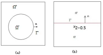
together with Dirichlet conditionsu=g(x)on the boundary of the regionΩ = Ω+∪Ω−∪Γ(shown as Fig. 1), Γis the intersection curve (called as interface) of the subregionsΩ+ andΩ−whereφ(x)>0andφ(x)<0, respectively, and the equation of the interface is φ(x) = 0,β(x)is a continuous function.
On the interface, jump conditions are as follows
[u]|Γ = (u+−u−)|Γ=g0(x), (2)
[∂u
∂n]|Γ= (u
+ n −u
−
n)|Γ=g1(x), (3) whereu+, u− andu+n, u−n are the solutions onΩ+,Ω− and the outer normal derivatives onΓ, respectively.
IAENG International Journal of Applied Mathematics, 47:3, IJAM_47_3_05
Fig. 1. The region and the interfaces.
If problem (1) satisfies the compatibility condition
−
Z
Γ
g1ds=
Z
Ω
f(x)dx,
then there exists unique solution for it.
To solve problem (1), one agreeable idea is to transform it to another elliptic problem with the natural jump condition
[q]|Γ = 0,[qn]|Γ= 0, (4)
where
q(x) =u(x)−uˆ(x), (5)
ˆ
u(x) =
0, x∈Ω− , ˜
u(x), x∈Ω+, (6)
andu˜(x)is the undetermined smooth function.
From (5) and (6), problem (1) can be transformed as follows
−∇ ·(∇q) = ˜f , x∈Ω/Γ, (7) [q](x) = 0, x∈Γ,
[qn](x) = 0, x∈Γ,
q(x) =q0, x∈∂Ω,
wheref˜=
f−, x∈Ω−,
f++4u˜(x), x∈Ω+, andq0= (g−u˜)|∂Ω.
One can see that (7) is an usual elliptic problem convenient to be solved by many numerical methods. Hence, it is the key point to construct the normal extended function u˜(x) according to compulsory conditions (2) and (3) in interface problems. It is our main task to take in this paper.
III. CONSTRUCTION OF THE NORMAL EXTENDED FUNCTION
We will come to discuss how to extend the functiong0(x) in (2) to some given subregion, such as Ω+, in the normal direction. Let the extended function be u˜(x). From (2),(3) and (4), we can obtain
˜
u|Γ+=g0(x), (8)
˜
un|Γ+ =g1(x), (9)
[image:2.595.316.536.55.134.2]whereΓ+ means the single side limit from subregionΩ+. In the following, we shall present how to construct u˜(x) with the compulsory conditions (8) and (9) according to open and closed interface curves, respectively.
Fig. 2. A special interface.
A. Open interface curve
We firstly derive the normal extent function u˜(x) for a simple but basic interface curveΓexpressed asφ(x) =x2−
x1 = 0. Let s= x2√−2x1, t= x2√+x21 andu˜ be in the form of power series
˜
u(x) = ˜u(s, t) =
∞
X
i=0
ai(t)si, (10)
where the interfaceΓ :s= 0and variabless, tare shown in Fig. 2 (a).
To obtain u˜, we only need determine the coefficients
ai(t), i= 0,1,2,3, ....
The conditions (8) and (10) lead to
a0(t) = ˜u|s=0=g0(x(t)). (11)
By some basic calculations and conditions (9) and (10),
a1(t) =∂u˜
∂s|s=0=un|Γ+ =g1(x(t)). (12)
From some inductions, one can see that
−4u˜=−4˜u,˜ (13)
where4˜u˜= ∂∂s2u2˜+ ∂2u˜ ∂t2,4u˜=
∂2u˜ ∂x2 1
+∂∂x2u˜2 2 . From (14) and the facts
−4˜u˜|Γ = [−
∞
X
i=0
a”i(t)si+
∞
X
i=2
aii(i−1)si−2]|s=0
= −a”0(t)−2a2,
and
−4˜u|Γ =−4(u+−u−)|Γ = (f+−f−)|Γ,
one can obtain
a2(t) =− 1 2a
” 0(t)−
1 2!(f
+
−f−)|s=0,
wherea” 0(t) =
∂2a 0 ∂t2 , and(f
+−f−)|
s=0is a function about variablet.
Similar derivation leads to
a3(t) =−1
6a ” 1(t)−
1 3!
∂(f+−f−)
∂s |s=0.
In general,
ak(t) =− 1
k(k−2)a ” k−2(t)−
1
k!F
(k−2)(t), k
≥2, (14)
wherea” k−2(t) =
∂2ak−2 ∂t2 ,
and F(k−2)(t) := ∂k−2∂(fk−+2−sf−)|s=0 is a function about variablet.
IAENG International Journal of Applied Mathematics, 47:3, IJAM_47_3_05
[image:2.595.269.549.257.796.2]Hence, from (11), (12) and (15), we have
ak(t) =
g0(x(t)), k= 0,
g1(x(t)), k= 1,
− 1
k(k−1)a ” k−2(t)−
1 k!F
(k−2)(t), k≥2, (15)
and the normal extended correction function (10) is deter-mined.
Remark 1: We can obtain the corresponding extended func-tion only by some rotafunc-tion transformafunc-tion as the interface is other straight line.
In the following, we will consider a general case. In general, we can consider the interface composed by sev-eral segment lines. To be convenient, we only discuss the case of two segment lines (shown as Fig. 2 (b)), where Γ = Γ1∪Γ2, (x10, x02) = Γ1∩Γ2, and
Γ1: x2=x02, x1≥x01, Γ2: x1=x01, x2≤x02.
Hence, regionΩis divided into two subregionsΩ−andΩ+, andΩ+ is partitioned three parts Ω+,i, i= 1,2,3.
Assume that interface functionsg0(x), g1(x), x∈Γ1,Γ2, are smooth enough, respectively. In the following, we shal-l determine the corresponding normashal-l extended functions ˜
ui(x), i= 1,2,3 in three subregions, respectively. For the interface Γ1:x2−x02= 0,
˜
u1(x) =
∞
X
i=0
ai(x1)(x2−x02)
i, x∈Ω+,1. (16)
By some calculations similar to (15),
ak(x1) =
g0(x1), k= 0,
g1(x1), k= 1,
− 1
k(k−1)a ”
k−2(x1)− 1 k!F
(k−2)(x1), k≥2,
where
F(k−2)(x1) =
∂k−2(f+−f−)
∂xk2−2 |x2=x02
= ∂
k−2(f+−f−)
∂xk2−2 (x1).
For the interface Γ2:x1−x01= 0,
˜
u2(x) =
∞
X
i=0
bi(x2)(x1−x01)
i, x∈Ω+,2. (17)
Similarly, we have
bk(x2) =
g0(x2), k= 0,
g1(x2), k= 1,
− 1
k(k−1)a ”
k−2(x2)− 1 k!F
(k−2)(x2), k≥2,
where
F(k−2)(x2) = ∂
k−2(f+−f−)
∂xk1−2 |x1=x01
= ∂
k−2(f+−f−)
∂xk1−2 (x2).
For the remainder subregion Ω+,3, we can choose the simplest way that the normal extended function is a constant
g0(x01, x02). This way naturally satisfies the consistency of t-wo normal extended functions defined in subregions between Ω+,1 andΩ+,2.
˜
u3(x) =g0(x01, x 0
2), x∈Ω +,3
. (18)
Hence, the normal extended function u˜(x),x ∈ Ω+ is completely determined by (16), (17) and (18) for this general case.
Remark 2: We maybe encounter some difficulties when the reconstructions are needed for the first, even second order derivative at some non-interface point by u˜3(x),x∈Ω+,3. These difficulties are from the facts that the derivative function is discontinuous on the intersection face between subregions Ω+,3 and Ω+,i, i = 1,2. In practice, we can use some smooth curves to approximate the corner(x01, x02), which can relieve even eliminate it.
B. Closed interface curve
We firstly consider a simple but basic case that the interface is consisted of a rectangle (shown as 2 (c)). We shall not present the derivation and construction of the normal extended function u˜(x),x ∈ Ω+ because its procedure is only to repeat and resemble that in Section 3.1. As a matter of fact, we can deal with some convex closed polygon interface only by some rotation transformation.
In the following, we will consider how to construct the normal extended functionu˜(x),x∈Ω+ when the interface is a circle
r=r0,
wherer=px2
1+x22 andr0 is a constant.
Let u˜(x),x ∈ Ω+ be the form of power series in polar coordinates
˜
u(x) = ˜u(r, θ) =
∞
X
i=0
ai(θ) (r−r0)i, (19)
whereθ= arctan(x2 x1). Firstly, we have
a0(θ) = ˜u|r=r0=g0(r0, θ),
a1(θ) = ∂u˜
∂n|r=r0 =
∂u˜
∂r|r=r0 =g1(r0, θ). Noticing that
4u˜|Γ = ( 1
r ∂u˜
∂r + ∂2u˜
∂r2 + 1
r2
∂2u˜
∂θ )|Γ
= 1
ra1(r0, θ) + 2!a2(r0, θ) +
1
r2a 00 0(r0, θ)
= (f+−f−)|Γ,
we have
a2(θ) =− 1 2![(f
+−f−)|
Γ+ 1
r0
a1(r0, θ) + 1
r2 0
a000(r0, θ)].
In general, fork≥2,
ak(θ) = − 1
r2 0
1
k(k−1)a ”
k−2(r0, θ)− 1
r0 1
ka
0
k−1(r0, θ)
−1
k!Fk−2(r0, θ),
whereFk(r0, θ) =
∂k−2(f+−f−) ∂rk−2 |Γ1. Hence, we have
ak(θ) =
g0(r0, θ), k= 0,
g1(r0, θ), k= 1,
−1 r2 0
1 k(k−1)a
”
k−2(r0, θ)−r101ka 0
k−1(r0, θ)
− 1
k!Fk−2(r0, θ), k≥2,
IAENG International Journal of Applied Mathematics, 47:3, IJAM_47_3_05
where
F(k−2)(r0, θ) =
∂k−2(f+−f−) ∂rk−2 |Γ
= ∂
k−2(f+−f−)
∂rk−2 (r0, θ).
Therefore, the normal extended function (19) is deter-mined.
Remark 3: For the general interface curveΓ :φ(x) = 0, let ˜
ube in the form of generalized power series as follows
˜
u(x) =
∞
X
i=0
ai(x)φi(x).
Due to the complicity, we only roundoff it several terms to approximate the normal extended function u˜. For instance, we have
˜
u(x)≈a0(x) +a1(x)φ(x) +a2(x)φ2(x),
where
a0(x) =g0(x), a1(x) = 1 ∂φ ∂n
(g1−
∂g0
∂n)|φ(x)=0,
a2(x) =
(f+−f−)− 4g
0−g14φ−2∇g1· ∇φ 2!|∇φ|2 |φ(x)=0.
IV. AN ALGORITHM FOR THE NORMAL EXTENDED FUNCTION
To construct the normal extended function, we present an algorithm about how to obtain the corresponding coordinates on the interface for any point in the extended region. After acquiring the coordinates, we can get the values at non-interface point.
Algorithm 1:
Input: any pointP(x1, x2)∈Ω+ and the interface level-set functionφ(x1, x2).
Output:P0(x01, x02)∈Γ.
Conditions: −−→P0Pkn, where n is the out normal vector at
P0.
Step 1: find the equation of the line:−−→P0P
x01−x1
φx1(x 0 1, x02)
= x 0 2−x2
φx2(x 0 1, x02)
, (20)
where
φx1(x 0 1, x
0 2) =
∂φ(x)
∂x1
|(x0 1,x02),
φx2(x 0 1, x
0 2) =
∂φ(x)
∂x2
|(x0 1,x02).
Step 2: solve the equation (20) with the following one simultaneously,
φ(x01, x02) = 0,
then we can get the corresponding coordinates (x0 1, x02) on the interface.
Remark 4: In above algorithm, the iterative methods, such as the fixed point method or Newton iterative method, are always introduced to solve the nonlinear equations.
V. NUMERICAL EXPERIMENTS
In this section, we will present two typical numerical examples for normal extended functions when the interface curves are open and closed, respectively, as solving interface problem (1). In numerical tests, the linear finite element method is employed, we only choose some parts of the power series which are enough to obtain the saturated convergent order of finite element approximations for interface problem (1) in our tests.
Example 1 In problem (1), we choose β+ = 1, β− = 2,
Ω = (0,1)2, the interfacex
2−0.5 = 0and
u(x) =
u+= 2sin(πx1)sin(πx2)(x2−0.5), x∈Ω+,
u−=sin(πx1)sin(πx2)(x2−0.5) + 2, x∈Ω−. One can see that
[u]|Γ=−2, [un]|Γ= 0.
We choose the interceptive (roundoffed) normal extended function u˜(x) = −2 in this problem and carry on with the numerical tests as follows. Numerical results are shown as Tab. 1, where k · kς, ς = 0,1,∞ denote the norms
L2, H1, L∞, and γ denotes the ratio of the errors u−uh between the step sizeshandh2. From the results in this table, one can see that the errors ofuh in normsL2, H1, L∞ are
saturated-convergence orders, respectively.
TABLE I
THE ERRORS OFuhIN NORMSL∞, L2, H1FOR THE OPEN INTERFACE
CURVE.
N1×N2 ku−uhk0 γ ku−uhk∞ γ ku−uhk1 γ
8×8 3.3005e-3 6.95e-2 2.55
16×16 8.7057e-4 4.00 2.23e-2 3.12 1.32 1.93
32×32 2.2394e-4 4.00 5.69e-3 3.92 6.69e-1 1.97
64×64 5.6827e-5 4.00 1.43e-3 3.98 3.39e-1 1.97
Example 2 In problem (1), we choose (as reference [2]) β+ =β− = 1, the interface x2
1+x22 =r20,r0 = 0.5, Ω = (−1,1)2 and
u(x) =
2r3+ 5, φ(x)≤0,
r3, φ(x)>0, r=
q
x2 1+x22.
One can see that
[u]|Γ =−(r30+ 5), [un]|Γ=−3r20.
We choose the interceptive (roundoffed) normal extended function is
˜
u(x) =−(r30+ 5)−3r20 r
2−r2 0 2r ,
in this example and carry on numerical tests as follows. Numerical results are shown as Tab. 2 . From the results in this table, one can see that the errors of uh in norms
L2, H1, L∞ are saturated-convergence orders, respectively.
VI. SUMMARY AND CONCLUSIONS
In this paper, we construct the normal extended correction function in the form of power series which are helpful to theoretical analysis, for open and closed interface curves, respectively. A simple but basic and efficient algorithm is designed to obtain the extended function value of
IAENG International Journal of Applied Mathematics, 47:3, IJAM_47_3_05
TABLE II
THE ERRORS OFuhIN NORMSL∞, L2, H1FOR THE CLOSED
INTERFACE CURVE.
N ku−uhk0 γ ku−uhk∞ γ ku−uhk1 γ
64 3.989e-5 1.636e-4 1.506e-1
128 1.204e-5 3.23 4.779e-5 3.43 7.533e-2 1.99
256 2.872e-6 4.19 1.162e-5 4.11 3.767e-2 1.99
512 7.261e-7 3.95 2.973e-6 3.91 1.884e-2 1.99
1024 1.769e-7 4.10 7.327e-7 4.06 9.421e-3 1.99
any non-interface point projected to the interface in the direction of normal direction. We apply the extended function to some interface problems and carry on some numerical experiments. Numerical results confirm the validity of normal extended functions and the efficiency of the algorithm. In the future, we will consider the following two problems: one is how to reconstruct the corresponding first and second order derivatives by the normal extended function values, the other is how to construct the normal extended function for some interface curves which are not convex. For the second one, maybe we can only design some algorithm for some neighbor region near the interface curve or else the projected interface point can not uniquely be determined. These are main tasks in the future.
Acknowledges
The authors thank the referees for their valuable sugges-tions to improve this paper greatly and are also grateful to Professor S. Shu for some helpful discussions on numerical experiments.
REFERENCES
[1] S. H. Chou, D. Y. Kwak, and K. T. Wee, “Optimal Convergence Analysis of an Immersed Interface Finite Element Method,”Advances in Computational Mathematics, vol. 33, no. 2, pp149-168, 2010 [2] R. J. LeVeque, and Z. L. Li, “The Immersed Interface Method for
Ellip-tic Equations With Discontinuous Coefficients and Singular Sources,”
SIAM Journal on Numerical Analysis, vol. 31, no. 4, pp1019-1044, 1994 [3] S. Y. Kadioglu, R. R. Nourgaliev, and V. A. Mousseau, “A Compar-ative Study of the Harmonic and Arithmetic Averaging of Diffusion Coefficients for Non-linear Heat Conduction Problems,”Idaho National Laboratory, March, 2008
[4] C. Y. Nie, and H. Y. Yu, “A Novel Finite Volume Scheme with Geometric Average Method for Radiative Heat Transfer Problems,”
Applied Physics Frontier, vol. 1, no. 4, pp32-44, 2013
[5] Lingzhi Qian, and Huiping Cai, “Two-grid Method for Characteristics Finite Volume Element of Nonlinear Convection-dominated Diffusion Equations,”Engineering Letters, vol. 24, no. 4, pp399-405, 2016 [6] Miaochan Zhao, Hongbo Guan, and Pei Yin, “A Stable Mixed Finite
Element Scheme for the Second Order Elliptic Problems,” IAENG International Journal of Applied Mathematics, vol. 46, no. 4, pp545-549, 2016
[7] S. Hou, and X. D. Liu, “A Numerical Method for Solving Variable Co-efficient Elliptic Equation With Interfaces,”Journal of Computational Physics, vol. 202, no. 2, pp411-445, 2005
[8] A. Wiegmann, and K. P. Bube, “The explicit-jump immersed interface method: finite difference methods for PDES with piecewise smooth solutions,”SIAM Journal on Numerical Analysis, vol. 37, no. 3, pp827-862, 2000
[9] J. Wang, “Asymptotic expansions andL∞-error estimates for mixed finite element methods for second order elliptic problems,”Numerische Mathematik, vol. 55, no. 4, pp401-430, 1989
[10] I. Klapper, and T. shaw, “A large jump asymptotic framework for solving elliptic and parabolic equtions with interfaces and strong coefficient discontinuities,”Applied Numerical Mathematics, vol. 57, no. 5, pp657-671, 2007
[11] C. Y. Nie, and H. Y. Yu, “Some error estimates on the large jump asymptotic method for parabolic interface problems,”Applied Mechan-ics and Materials, vol. 126, pp4726-4731, 2012
[12] C. Y. Nie, and H. Y. Yu, “Some error estimates on the large jump asymptotic approach for the interface problem,”Applied Mathematics and Computation, vol. 263, pp268-279, 2015
[13] Z. Sadati, “Numerical Implementation of Triangular Functions for Solving a Stochastic Nonlinear Volterra-Fredholm Integral Equation,”
IAENG International Journal of Applied Mathematics, vol. 45, no. 2, pp102-107, 2015