A novel approach to quantify and analyse brain imaging features on MRI

A novel approach to quantify and

analyse brain imaging features on MRI

Myriam Jaarsma-Coes, 31 august 2017

Graduation committee

Chairman and Technical supervisor University of Twente

Prof.dr.ir. C.H.Slump Robotics and Mechatronics

University of Twente, Enschede, The Netherlands

Medical supervisor Dr. J. de Bresser

Department of Radiology

Leids Universitair Medisch Centrum, Leiden, The Netherlands Universitair Medisch Centrum Utrecht, Utrecht, The

Netherlands Technical supervisor UMC Utrecht I. Kant, MSc.

Department of Radiology & Intensive Care Medicine Universitair Medisch Centrum Utrecht, Utrecht, The Netherlands

Process supervisor Drs. P.A. van Katwijk

Master’s program Technical Medicine

University of Twente, Enschede, The Netherlands

External member J.K. van Zandwijk, MSc.

Master’s program Technical Medicine

University of Twente, Enschede, The Netherlands

Additional member Prof.dr. J. Hendrikse

Department of Radiology

Acknowledgements

After eleven month of working on my thesis, today is the day: writing this note of thanks, the finishing touch of my thesis. It has been a period of intense learning for me, not only in the scientific arena, but also on a personal level. I would like to shortly reflect on the people who supported my growth towards the technical medicine physician I am today.

I would like to express the deepest appreciation to Jeroen de Bresser, for all his guidance, the interesting scientific discussions and patience. Special thanks to Kees Slump, for his critical questions and feedback especially on the technical part of this thesis. You helped to give my thesis more technical body. I would like to express my gratitude to Paul van Katwijk and my fellow intervision group members (Eline, Lennert and Luca) for listening and asking good questions to help me grow as a person. Paul, your questions and feedback always were spot on and gave me interesting insights. I have greatly benefited from Ilse Kant, I would not only like to thank you for your help on the technical part of this thesis but also for the fact that you always made time for me when my head was full, then you patiently listened to me and asked the right questions. I would also like to give thanks to Jeroen Hendrikse and Jordy van Zandwijk for making my thesis and graduation possible. Special thanks also to Hugo Kuijf, Mirjam Geerlings and Rashid Ghaznawi for the data and their collaboration, feedback, help with the statistics and interesting questions. I received generous support from everyone working at the radiology department, especially during my radiology internship when they always made time for guidance and discussing findings. Finally, I would like to thank all the researchers in Q2 for their scientific input, sociability during lunch breaks and our games of table soccer.

I owe my deepest gratitude to my parents for their wise counsel and sympathetic ear, you are always there for me. I would like to thank my brother, sister and friends for the necessary distractions, sociability and a listening ear. And last, but surely not least, I would like to thank Ruben for all the support, love and so much more!

Contents

Graduation committee i

Acknowledgements iii

Contents v

List of figures vii

List of tables ix

List of Abbreviations xi

Summary 1

1 Shape feature analysis method for WMH: development, description and assessment 3

1.1 Abstract 4

1.2 Introduction 5

1.3 Methodology 6

1.3.1 Requirements 6

1.3.2 Shape measures 6

1.3.3 Descriptor validation 9

1.3.4 Descriptor evaluation 9

1.4 Experimental results 11

1.4.1 Descriptor validation 11

1.4.2 Descriptor evaluation 11

1.4.3 Shape descriptors in the SMART-MR cohort 13

1.5 Discussion and conclusion 18

2 Different brain imaging phenotypes in patients with manifest arterial disease 19

2.1 Abstract 20

2.2 Introduction 21

2.3 Materials and methods 22

2.3.1 Study population 22

2.3.2 Magnetic resonance imaging protocol 22

2.3.3 Brain MRI markers 22

2.3.4 Cardiovascular risk factors 24

2.3.5 Cluster analysis 24

2.3.6 Statistical analysis 24

2.4 Results 25

2.5 Discussion 34

Bibliography 37

Appendix A. Shapes used for descriptor evaluation. 41

Appendix B. Results shape features on shape range. 43

List of figures

Figure 1. The major and minor axis 8

Figure 2. Example of a surface with surface normal 𝑵 and principal curvatures 𝒌1 & 𝒌2 8 Figure 3. U shapes with varying sizes, orientations and with and without gaps. 10

Figure 4. Spheres with varying diameters and orientations. 10

Figure 5. Cantor dust in 2D and 3D. 10

Figure 6. The four selected shape descriptors set out against the log transformed volume. 13

Figure 7. Convexity versus solidity plot with WMH visualization 15

Figure 8. Fractal dimension versus concavity index plot with WMH visualization 16

Figure 9. Eccentricity 17

Figure 10. The dendogram combined with a heatmap of the 17 input parameters. 27

Figure 11. Two CPWMH lesions (red) in two patients 27

Figure 12. The chance of WMH and BPF presence per cluster in the three cluster approach. 32 Figure 13. The chance of WMH and BPF presence per cluster in the seven cluster approach. 33 Figure 14. Fifteen confluent lesions (A) and thirteen periventricular lesions (B) used for descriptor

validation. 41

Figure 15. Eleven deep lesions used for descriptor validation. 42

List of tables

Table 1. Evaluation of area, volume, convex area, convex volume and box count measurements. 11 Table 2. Evaluation of axis length and eccentricity measurements. 11 Table 3. Evaluation of the fractal dimension by using objects with known fractal dimensions. 11

Table 4. Results from the shape descriptor evaluation. 12

Table 5. Shape descriptors calculated for the cluster analysis 23

Table 6. Demographics and clinical characteristics of the total cohort and clusters identified by cluster

analysis. 26

Table 7. Description of the total cohort and clusters identified by cluster analysis 26 Table 8. Demographics and clinical characteristics of seven clusters identified by cluster analysis. 28 Table 9. Description of the seven clusters identified by cluster analysis 29

Table 10. The optimal clustering method. 46

Table 11. The best number of clusters. 47

List of Abbreviations

AAA Abdominal aortic aneurysm

AD Average distance

ADM Average distance between means

ALVIN Automated lateral ventricle delineation APN Average proportion of non-overlap

BMI Body mass index

CADASIL cerebral autosomal dominant arteriopathy with subcortical ischemic strokes and leukoencephalopathy

CARASIL cerebral autosomal recessive arteriopathy with subcortical ischemic strokes and leukoencephalopathy

CPWMH Confluent and periventricular white matter hyperintensities

CSF Cerebral spinal fluid

CSVD Cerebral small vessel disease

CWMH Confluent white matter hyperintensities

DM Diabetes mellitus

DWMH Punctuate white matter hyperintensities

FD Fractal dimension

FLAIR Fluid attenuating inverse recovery

FOM Figure of merit

GMF Cortical grey matter fraction

HC Hierarchical clustering

ICV Intracranial volume

IMT Intima-media thickness

IR Inversion recovery

k-NN k-nearest neighbours

LVD Large vessel disease

MR Magnetic resonance

MRI Magnetic resonance imaging

PCA Principle component analysis

PVWMH Periventricular white matter hyperintensities

QQ quantile-quantile

SD Standard deviation

SMART-MR Second Manifestations of ARTerial disease - Magnetic Resonance

SVD Small vessel disease

T Tesla

TE Echo time

TI Inversion time

TR Repetition time

VF Ventricle fraction

WMF White matter fraction

WMH White matter hyperintensities

Summary

Atherosclerosis is a progressive inflammatory artery disease responsible for about 50% of deaths in the western world, mainly due to heart disease and stroke [1], [2]. Brain abnormalities that can be seen in patients with arterial disease (atherosclerosis) are heterogeneous and are the result of different underlying etiologies. The three main groups of brain abnormality etiologies are neurodegenerative disease, large vessel disease and small vessel disease.

The main neuroimaging feature of neurodegenerative disease are localized (hippocampal, temporal, frontal and parietal) and global atrophy while large vessel disease (LVD) leads to cortical infarcts. Neuroimaging features of cerebral small vessel disease (CSVD) include: recent small subcortical infarcts, lacunar infarcts, white matter hyperintensities (WMH), dilated perivascular spaces, cerebral microbleeds and possibly even brain atrophy [3]. CSVD results from a complex mix of genetic and cardiovascular risk factors [4]. There are several types of CSVD based on etiology (most common are arteriolosclerosis, cerebral amyloid angiopathy and genetic SVD)[5]. These different types of CSVD may lead to different manifestations of imaging features of CSVD.

1.1

Abstract

WMH exhibit large inter-individual variability in terms of regional distribution, severity, rate of

1.2

Introduction

Cerebral small vessel disease (CSVD) is involved in one-third of ischemic strokes and more than 90% of intracerebral haemorrhages and contributes significantly to cognitive decline and dementia in the elderly [5], [6]. Even though CSVD is a serious healthcare issue, it has only gained more interest over the past 20 years.

The pathogenesis of CSVD is still largely unknown [7]. The main mechanism underlying SVD-related brain injuries is usually assumed to be ischemia. However, ischemia caused by arteriolar occlusion might be a late-stage phenomenon caused by endothelial damage. This damage can lead to passage of plasma proteins into the vessel wall, damaged vessel walls [8], leakage of fluid [9], albumin [10], other plasma proteins, and inflammatory cells [11] causing damage in the white and deep grey matter. CSVD results from a complex mix of genetic and cardiovascular risk factors, the most important of which are age and hypertension [4]. Neuroimaging features of CSVD include recent small subcortical infarcts, lacunes of presumed vascular origin, white matter hyperintensities (WMH) of vascular origin on T2/FLAIR MRI, dilated perivascular spaces cerebral microbleeds and brain atrophy [3], [5] .

Although WMH are commonly found in healthy elderly people, WMH are commonly related to cerebrovascular disease, cardiovascular disease, dementia and psychiatric disorders [12]–[14]. WMH exhibit large inter-individual variability in terms of regional distribution, severity, rate of progression and clinical consequences [15].

Currently, the WMH burden is mainly expressed in terms of volume [3] and lacks the potential to explain this large inter-individual variability. Shape and localization of WMH are potential discriminating features [16]–[18]. For example, cerebral autosomal dominant arteriopathy is associated with WMH located in the temporal lobe, whereas cerebral amyloid angiopathy is associated with WMH located in the posterior lobe [19]–[21]. WMH can be divided into periventricular (PVWMH) and deep (DWMH) [22] or in three subtypes PVWMH, DVWMH and confluent WMH (CWMH) [23], [24]. Differentiation between PVWMH, CWMH and DWMH is based on the distance to the lateral ventricles [25]. Post-mortem studies showed that PVWMH show signs of non-ischemic damage; discontinuous ependymal, gliosis, loosening of the white matter fibres and myelin loss, whereas DWMH show signs of chronic small vessel disease[15], [23], [26]. In a review on WMH, Kim et al. [23] concluded that smooth PVWMH are linked to an increase of interstitial fluid, whereas irregular PVWMH/CWMH are more likely caused by hypo perfusion and, DWMH are more related to small vessel disease.

It is challenging to assess and quantify WMH shape visually. Therefore, algorithms that can automatically assess WMH shape descriptors need to be developed. No studies were found that performed shape analysis of WMH of vascular origin. However, in other research fields shape descriptors as eccentricity, convexity, solidity, compactness, fractal dimension, curvedness and shape index have been used to discriminate between different types of lesions [27]–[33].

1.3

Methodology

1.3.1

Requirements

The requirements imposed on the shape descriptors are:

1. Independence of volume, volume should not solely influence the outcome. 2. The outcomes of the shape descriptors should be distributed evenly:

a. No flooring effect b. No ceiling effect

c. Preferably: Distributed normally, to facilitated statistical analysis d. Preferably: The values of the shape ranges between 0 and 1 3. Robustness,

a. Positioning of the lesions should not influence the outcome, shape measures should be: i. Rotational invariant

ii. Scaling invariant iii. Translational invariant

b. Should perform well with limited resolution

4. Preferably: Interpretation should be straight forward and comprehensible for clinicians.

1.3.2

Shape measures

The WMH shape descriptors can be divided into area based (surface area, convexity, surface index and curvature), dimension/volume based (volume, solidity, complexity, eccentricity and fractal dimension). These descriptors are calculated from the binary segmented data.

Volume is a quantification of a 3D space enclosed by a surface. WMH volume is used to calculate the solidity (equation 1.4), complexity (1.12) and compactness (1.13) of the lesions and is used as a parameter to express the WMH load. Volume is defined as:

𝑉𝑜𝑙𝑢𝑚𝑒 = 𝑛 ∙ 𝑥𝑥𝑦𝑧 1.1

With 𝑛 as the number of voxels and 𝑥𝑥𝑦𝑧 as the voxel size.

Surface area is the size of the lesion interface so the surface of the enclosed 3D space. The surface area is used to calculate the convexity (equation 1.3), complexity (1.12) and compactness (1.13) of the lesions. Area is defined as:

𝐴𝑟𝑒𝑎 = (𝑓_{𝑒𝑥𝑝𝑥𝑦}+ 𝑓_{𝑒𝑥𝑝−𝑥𝑦}) ∙ 𝑥𝑥𝑦+ (𝑓_{𝑒𝑥𝑝𝑥𝑧}+ 𝑓_{𝑒𝑥𝑝−𝑥𝑧}) ∙ 𝑥𝑥𝑧 + (𝑓_{𝑒𝑥𝑝𝑦𝑧}+ 𝑓_{𝑒𝑥𝑝−𝑦𝑧}) ∙ 𝑥𝑦𝑧 1.2

𝑓𝑒𝑥𝑝 is defined as the number of voxel faces exposed in the indicated direction and 𝑥 the voxel size in the indicated direction.

The size and shape of concavities seems different between the WMH of different subjects. An object with more concavities has a higher jaggedness of edges. This is a measure for roughness, as the surface has more concavities the area increases and volume decrease and therefore the roughness increases. Solidity and convexity describe roughness by the extent to which the shape is convex or concave. A fully convex shape has a convexity of 1.

Even though convexity and solidity have not been used to analyses WMH other field have used these to analyses shapes. Lui et al. shows that a combination of solidity and convexity can be used to distinguish shapes based on number, shape and size of concavities for volcanic ash analysis [32].The convexity will decrease as the shape becomes more concave.

The convexity is defined as:

𝐶𝑜𝑛𝑣𝑒𝑥𝑖𝑡𝑦 =𝐴𝑟𝑒𝑎 𝑐𝑜𝑛𝑣𝑒𝑥 ℎ𝑢𝑙𝑙_{𝐴𝑟𝑒𝑎} 1.3

Solidity is defined as:

A shape or set of points is convex if for any two points that are part of the shape, the whole connecting line segment is also part of the shape. The convex hull is the smallest convex set that contains the subset or shape. [34]

The solidity and convexity can be combined using formula 1.5 to obtain the concavity index.

𝐶𝑜𝑛𝑐𝑎𝑣𝑖𝑡𝑦 𝐼𝑛𝑑𝑒𝑥 = √(1 − 𝑠𝑜𝑙𝑖𝑑𝑖𝑡𝑦)2_{+ 2 − 𝑐𝑜𝑛𝑣𝑒𝑥𝑖𝑡𝑦}2 _1.5 The fractal dimension is not previously used to analyse WMH but is already been used to quantify grey matter [30] and white matter [31] morphometric variability (complexity). Fractal objects are defined as scale-invariant (self-similar or self-affine). A fractal is an assemblage of rescaled copies of itself. Self-similarity occurs when the object is scaled in all direction where self-affinity occurs when scaled anisotropic. The fractal dimension measures the textural roughness of an object. The higher the fractal dimension the more irregular the object compared to a lower dimension. An object with a fractal dimension between 2 and 3 fills more space than a surface but less space than a volume. Box-counting was used as it can be applied in any dimension and with or without self-similarity. [35], [36] The fractal dimensions is defined as [37]:

𝐹𝑟𝑎𝑐𝑡𝑎𝑙 𝑑𝑖𝑚𝑒𝑛𝑠𝑖𝑜𝑛 = lim

𝑟→1

log (𝑛𝑟)

log ( 1_{𝑟 )}

1.6

With 𝑛 as the number of boxes covered by the pattern and the inverse box size 1_𝑟 with 𝑟 = 2𝑝. The value of p ranges from the smallest p satisfying equation 1.7 till 0.

𝑙𝑒𝑠𝑖𝑜𝑛 𝑠𝑖𝑧𝑒𝑚𝑎𝑥 ≤ 2𝑝 1.7

We hypothesize that more benign WMH caused by oedema around the vessels is more ellipsoid and vascular damage more circular shaped. Eccentricity describes the deviation from a circle. The eccentricity of a circle is one and the eccentricity of a line is zero. Therefore, the eccentricity of an ellipse will be between zero and one. The eccentricity in this study is defined as [28]:

𝐸𝑐𝑐𝑒𝑛𝑡𝑟𝑖𝑐𝑖𝑡𝑦 =𝑀𝑖𝑛𝑜𝑟 𝑎𝑥𝑖𝑠_{𝑀𝑎𝑗𝑜𝑟 𝑎𝑥𝑖𝑠} 1.8

The major and minor axis (see figure 2) can be obtained by finding the eigenvector of the pixel coordinate values covariance matrix.

A non-singular 3𝑥3 matrix 𝑨has 3 eigenvalues 𝜆1, 𝜆2, 𝜆3 obtained by solving equation 1.9

|𝑨 − 𝜆𝑰| = 0 1.9

With

𝑨 = [

𝑣𝑎𝑟(𝑥) 𝑐𝑜𝑣(𝑥, 𝑦) 𝑐𝑜𝑣(𝑥, 𝑧) 𝑐𝑜𝑣(𝑥, 𝑦) 𝑣𝑎𝑟(𝑦) 𝑐𝑜𝑣(𝑦, 𝑧) 𝑐𝑜𝑣(𝑥, 𝑧) 𝑐𝑜𝑣(𝑦, 𝑧) 𝑣𝑎𝑟(𝑧) ]

1.10

The corresponding eigenvectors 𝒆1, 𝒆2, 𝒆3are obtained by solving equation 1.11:

(𝑨 − 𝜆𝑗𝑰)𝒆j= 0 1.11

Other shape descriptors that were investigated are defined below (equation 1.12-1.15). Such measures have previously been used to discriminate between malignant and benign tumours [27]–[29]. The roughness of a shape describes the extent of the irregularity of surface area. A regular object will have a lower roughness than an irregular object of the same volume, due to an increased area.

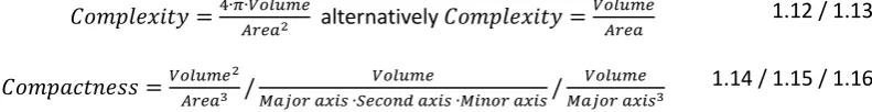
𝐶𝑜𝑚𝑝𝑙𝑒𝑥𝑖𝑡𝑦 =4∙𝜋∙𝑉𝑜𝑙𝑢𝑚𝑒_{𝐴𝑟𝑒𝑎2} alternatively 𝐶𝑜𝑚𝑝𝑙𝑒𝑥𝑖𝑡𝑦 =𝑉𝑜𝑙𝑢𝑚𝑒_{𝐴𝑟𝑒𝑎} 1.12 / 1.13

𝐶𝑜𝑚𝑝𝑎𝑐𝑡𝑛𝑒𝑠𝑠 =𝑉𝑜𝑙𝑢𝑚𝑒_{𝐴𝑟𝑒𝑎3}2/_{𝑀𝑎𝑗𝑜𝑟 𝑎𝑥𝑖𝑠 ∙𝑆𝑒𝑐𝑜𝑛𝑑 𝑎𝑥𝑖𝑠 ∙𝑀𝑖𝑛𝑜𝑟 𝑎𝑥𝑖𝑠}𝑉𝑜𝑙𝑢𝑚𝑒 /_{𝑀𝑎𝑗𝑜𝑟 𝑎𝑥𝑖𝑠}𝑉𝑜𝑙𝑢𝑚𝑒 ₃ 1.14 / 1.15 / 1.16 Other roughness based measures that were investigated include the shape index and curvedness. Shape index and curvedness are defined as [38]:

𝑆ℎ𝑎𝑝𝑒 𝑖𝑛𝑑𝑒𝑥 = _𝜋2𝑡𝑎𝑛−1𝒌1+ 𝒌2

𝒌1− 𝒌2

1.17

𝐶𝑢𝑟𝑣𝑒𝑑𝑛𝑒𝑠𝑠 = √𝒌12+ 𝒌22

1.18 Where 𝒌1 is the maximal curvature and 𝒌2 the minimal curvature (see figure 3), named the principal curvatures.

Figure 1. The major axis denotes the largest diameter of the lesions in 3D and minor axis denotes the smallest diameter of the lesions in 3D orthogonal to the major axis.

1.3.3

Descriptor validation

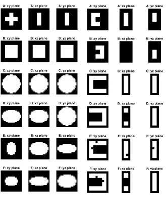
The performance of the previous described shape descriptors is examined using artificial shapes. Figure 3 shows six artificially created spheres with various axis lengths and orientations. Figure 4 shows six

artificially created u-shapes of various sizes, orientations and with and without gaps. Known volume, area, axis length and box counts are compared with the outcome of shape descriptors. Finally a line, plane, box and cantor dust were created to validate the fractal dimension measurement.

1.3.4

Descriptor evaluation

For this experiment a selection of lesions from previously generated WMH probability maps of the SMART-MR dataset were used (for more information see page 22). This selection was created in dialogue with a radiologist (JB).

Performance of the shape descriptors was evaluated using a selection of PVWMH, CWMH and DWMH lesions (for more information about lesion types see page 23). Lesions with different volumes were selected to represent the possible range in shape of the three lesion types. See Appendix A for

visualization of the shape ranges. Volume dependency was determined by plotting the shape descriptor versus the volume (sorted with ascending volume) of the lesions, a linear association was declared volume dependent. Spread, flooring and sealing effects were assessed in the same plots. For examination of the scale, translation and rotational invariance lesions were rotated, translated or scaled and outcomes of the shape parameters for the original shape and the rotated, translated or scaled lesions was

compared. Comprehensibility of these parameters for clinical practice was determined by a radiologist (JB).

Figure 4.3U shapes with varying sizes, orientations and with and without gaps.

Figure 5. Cantor dust in 2D and 3D.

Figure 3.4Sphereswith varying diameters

1.4

Experimental results

1.4.1

Descriptor validation

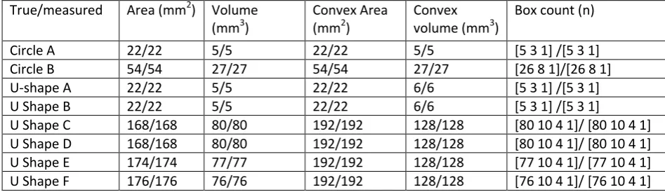
An overview of different results from the descriptor validation can be found in table 1, 2 and 3. All measurements of the synthetic lesions correspond to the true measures except for the estimation of the fractal dimension. Where a under estimation of the FD is present for the less complex figures (cube, plane and line) and a slight overestimation for cantor dust.

Table 1. Evaluation of area, volume, convex area, convex volume and box count measurements. True value/measured value

True/measured Area (mm2) Volume (mm3)

Convex Area (mm2)

Convex volume (mm3)

Box count (n)

Circle A 22/22 5/5 22/22 5/5 [5 3 1] /[5 3 1]

Circle B 54/54 27/27 54/54 27/27 [26 8 1]/[26 8 1]

U-shape A 22/22 5/5 22/22 6/6 [5 3 1] /[5 3 1]

U Shape B 22/22 5/5 22/22 6/6 [5 3 1] /[5 3 1]

U Shape C 168/168 80/80 192/192 128/128 [80 10 4 1]/ [80 10 4 1]

U Shape D 168/168 80/80 192/192 128/128 [80 10 4 1]/ [80 10 4 1]

U Shape E 174/174 77/77 192/192 128/128 [77 10 4 1]/ [77 10 4 1]

U Shape F 176/176 76/76 192/192 128/128 [76 10 4 1]/ [76 10 4 1]

Table 2. Evaluation of axis length and eccentricity measurements. True value/measured value

True/ measured First axis (mm) Second axis (mm) Third axis (mm) Eccentricity linear Eccentricity 321

Circle A 3/3 3/3 1/1 0.33/0.33 0.82/0.82

Circle B 3/3 3/3 3/3 1/1 0/0

Circle C 19/19 19/19 19/19 1/1 0/0

Circle D 19/19 19/19 13/13 0.68/0.68 0.56/0.56

Circle E 19/19 13/13 9/9 0.47/0.47 0.82/0.82

Circle F 19/19 13/13 9/9 0.47/0.47 0.82/0.82

Table 3. Evaluation of the fractal dimension by using objects with known fractal dimensions. True/measured (% difference)

Cube Plane Line 2D cantor 3D cantor

3/2.776(-7.5%) 2/1.833 (-8.3%) 1/0.951 (-4.9%) 1.678/1.690 (0.7%) 2.485/2.535 (2,0%)

1.4.2

Descriptor evaluation

The results of the descriptor evaluation are shown in table 4 These scores are based on the results of the parameters obtained from the selection of PVWMH, CWMH and DWMH lesions (see appendix B) and synthetic lesions (figure 3, 4 and 5).

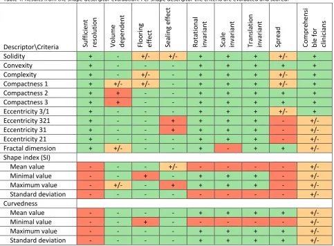
Some measures like fractal dimension, complexity and compactness measure similar shape characteristics. Because we are interested in unique characteristics of the lesions a comparative assessment was made. Even though the fractal dimension is not truly scale invariant this measure is chosen over complexity and compactness as these measures show some volume dependency and a more selective spread. This volume dependency is mostly caused by the fact that these are variants of the surface to volume ratio with is volume dependent. Moreover compactness 2 and 3 make use of the axis length obtained from the eccentricity calculation; due to the fact that PVWMH and CWMH are not spherical objects these measures are beside the point.

Solidity and convexity are used in further analysis due to the favourable characteristics. In contrast to other roughness measures are they not volume dependent and the spread is sufficient. Second of all, research into volcanic ash morphology [32] suggest that combining solidity and convexity can help distinguish between small and large concavities which is interesting when analysing PVWMH and CWMH lesions.

For shape index and curvedness measurements the resolution is not sufficient, therefore these measures will not be used further on in the clinical data analysis.

Table 4. Results from the shape descriptor evaluation. Per shape descriptor the criteria are evaluated and scored.

Descriptor\Criteria Suffic

ien t reso lu tio n Vo lu m e depend ent Flo o rin g ef fect Seali ng e ff ect Rot at io na l in var ia n t Sca le in var ia n t Tr an sla tio n in var ia n t Spre ad Co m pre h ens i bl e for clinicians

Solidity + - +/- +/- + + + +/- +

Convexity + - - - + + + + +

Complexity + - +/- - + + + +/- +

Compactness 1 + +/- +/- - + + + +/- +

Compactness 2 + + - - + + + + +

Compactness 3 + + - - + + + + +

Eccentricity 3/1 + - - - + + + +/- +

Eccentricity 321 + - - + + + + - +/-

Eccentricity 31 + - - + + + + - +/-

Eccentricity 21 + - - - + + + - +/-

Fractal dimension + +/- - - + - + + +/-

Shape index (SI)

Mean value - - - +/- - - +/-

Minimal value - - + - + + + - +/-

Maximum value - +/- - + + + + - +/-

Standard deviation - - - +/-

Curvedness

Mean value - - - - + + + + +/-

Minimal value - - + - - - +/-

Maximum value - - - - + + + + +/-

1.4.3

Shape descriptors in the SMART-MR cohort

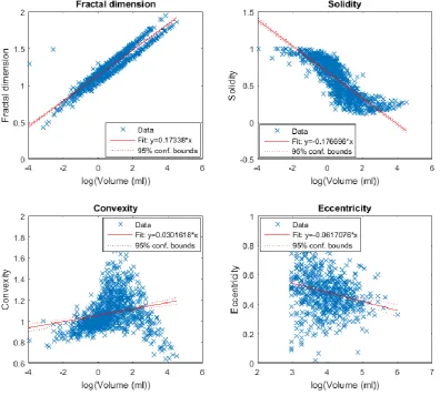
In the previous section four shape descriptors (fractal dimension, solidity, convexity and eccentricity) were selected as they satisfied most of the formulated criteria (see requirements, page 6 and table 4). In figure 6 the relation between WMH volume and the different shape descriptors is shown. The WMH volume is log transformed to obtain a normal distribution. Normality was conformed with a histogram and QQ plot. Fractal dimension and solidity are highly correlated with WMH volume (FD: r (9971) = 0.95, p < 0.001 & solidity: r (997) = -0.85, p < 0.001). Convexity and eccentricity have a weak correlation with WMH volume (Convexity: r (997) = 0.23, p < 0.001 & Eccentricity: r (632) = -0.24, p < 0.001).

Figure 6. The four selected shape descriptors set out against the log transformed volume. The WMH volume is log transformed to obtain a normal distribution. Increased WMH volume leads to an increase in fractal dimension and convexity while the solidity decreases. Eccentricity does not increase with volume.

1

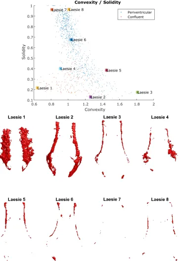
In figure 7 the convexity is plotted against the convexity for all CPWMH lesions to provide further insight into these descriptors. Lesions positioned in the left bottom corner are large and rough lesions with a large area and small volume compared to their convex hull. The lesions more to the right bottom still have a small relative volume, however their relative area decreases. Lesions with a higher solidity have a higher relative volume. Resulting in a shape that is more comparable to the convex volume, and therefore resulting in a more comparable area. Causing a more concentrated spread in convexity with higher solidities compared to low solidities (around Lesions 6, 7 and 8).

Figure 8 shows a plot of the fractal dimension versus the concavity index (a combination of solidity and convexity, see equation 1.5). It can be observed that an increase in volume and roughness also increases the fractal dimension of the lesions. This is in line with figure 6 in which a strong corrolation was shown between volume and fractal dimension. The concavity index, also a measure of roughness, can be used to differentiate between dense and irregular versus elongated and curved WMH.

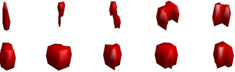
Figure 9 illustrates shapes of DWMH lesions with increasing eccentricity. Differences in eccentricity are difficult to assess visually. Indicating the additional value for shape descriptors in addition to volume and visual examination, on the other hand, it is also an indication that small changes in eccentricity may not be relevant.

1.5

Discussion and conclusion

In this study we investigated and evaluated possible shape descriptors for WMH lesions. This was done with the ultimate aim of providing additional discriminating information on outcome of patients with WMH and WMH etiology. First of all, we showed that shape descriptors of WMH can be calculated. When comparing area based, dimension/volume based and complex based shape descriptors we found that, convexity, solidity, eccentricity and fractal dimension meet most of the requirements outlined in table 4. Finally, shape descriptors were applied to WMH lesions of subject of the SMART-MR cohort. Even though the shape of the WMH lesions is highly correlated with WMH volume for some shape descriptors, findings suggest that shape measures can indeed provide additional information on different types of WMH with regard to irregularity.

During the validation of the shape descriptors we found that we can accurately measure volume, area and length of WMH lesions. However, this does not mean that our 3D shape descriptors for WMH are

completely accurate. For measuring the shape descriptors we are dependent on the voxel size and segmentation to obtain a digital representation of the WMH lesion. This limitation is especially of

influence on the accuracy in the SMART-MR data set as scans were made with an slice thickness of 4 mm. Resulting in limited data in the z-direction, the influencing the accuracy and precision of shape descriptor values of the smallest lesions the most.

The accuracy of our box-counting (table 3) method for 3D-FD calculation was good (with an maximal difference of 2%) for complex objects (2D and 3D cantor dust) and comparable to other published approaches to calculate the FD of the cerebral grey matter (difference 0.1 – 2%)[39]. However, for non-complex objects (cube, plane and line) the accuracy is low (maximal difference of 8.3%) compared to that reported by Esteban et al. [39]. This suggests that the FD for the PWMH and CWMH is thus more reliable than the FD for DWMH lesions, which are smaller and more cube or ellipsoid shaped.

Another possible limitation is that for the eccentricity we assumed that a deep WMH lesion is oval or round and thus the axis length are measured through the centre of the lesion, while in reality not all DWMH lesions are truly spherical.

Some measures can only be obtained using binary data (e.g. fractal dimension); while for other

descriptors it is also possible to assess the shape descriptors using a mesh. In this study all measures are calculated from binary images with the risk of losing the additional information of the probability values obtained by kNN classification (see brain segmentation, page 25). Meshes created with the marching cube algorithm on the probability maps might provide a more precise representation of the lesion resulting in even more reliable shape descriptors.

Possibilities for future research include assessing the reproducibility of the WMH shape descriptors by obtaining two datasets of the same subject within a short timeframe but in different scanning sessions using the same MRI scanner and protocol. Additionally it would be interesting to investigate the influence of resolution by scanning the same subject with different slice thicknesses. Quantification of the

variability caused by differences in slice selection, slice thickness and segmentation may increase our knowledge of the precision and accuracy of the shape descriptors. Furthermore, the relationship between WMH shape and WMH volume can be investigated more accurately. Finally and most importantly, it would be interesting to investigate the relation of WMH shape and clinical outcome (i.e. development of stroke, cognitive impairment or death). Like Artero et al. we found that WMH are most often localized in the frontal and parietal lobe. It would be interesting to investigate whether the shape of DWMH lesions is different per lobe.

2.1

Abstract

Objective: Brain abnormalities are heterogeneous and are the result of different underlying etiologies. These different etiologies can lead to different patterns of brain abnormalities that can be interpreted as different brain imaging phenotypes. We examined a cohort of patients with arterial disease and set out to identify subgroups with different brain imaging phenotypes using cluster analysis.

Method: We included 1003 patients with manifest arterial disease from the SMART-MR study. In these patients different brain imaging features were determined consisting of grey and white matter tissue volumes, presence of different types of brain infarcts and different features of white matter

hyperintensities (WMH). Hierarchical clustering was used to identify different subgroups based on these imaging features. To study the clinical relevance of these subgroups, the between group differences in patient characteristics and risk factors for vascular disease were examined.

Results: By cluster analysis 7 distinct groups of brain imaging phenotypes in patients with manifest arterial disease were found consisting of 28, 49, 118,120, 183, 205 and 300 patients. These groups were

significantly different in brain volumes, presence of different types of brain infarcts and different features of WMH (p<0.05). These groups can be interpreted as suffering from: small vessel disease (SVD) combined with cerebral atrophy, large vessel disease, intermediate cerebral atrophy and WMH, SVD and three relative healthy groups with low to intermediate cerebral atrophy and WMH. Groups were significantly different (p<0.05) in age, smoking, hypertension, hyperhomocysteinemia, diabetes, and in primary location of the manifest arterial disease.

Conclusions: Within a group of patients with arterial disease, we identified distinct brain imaging

phenotypes that were associated with different vascular risk factor profiles. This novel approach enables identification of different brain imaging phenotypes possibly associated with different still unknown underlying etiologies.

2.2

Introduction

Brain changes are heterogeneous and are the result of different underlying etiologies. The most frequent brain changes are neurodegenerative diseases, large vessel disease and cerebral small vessel disease. These brain changes are quite heterogeneous. CSVD for example has various underlying etiologies, the most common being arteriolosclerosis, cerebral amyloid angiopathy and genetic SVD (for example CADASIL2 and CARASIL3) [5]. However, even more unknown underlying etiologies might play an important role in the development of brain changes on MRI.

Specific neuroimaging features can reflect different etiologies. For example, subcortical infarcts resulting from large-vessel disease (LVD) are indistinguishable from those caused by SVD in the territory of the lenticulostriate arteries [40]. Furthermore, WMH are considered a neuroimaging feature of CSVD, but might not have an atheromatous etiology [41]. Nowadays research mainly focuses on solitary imaging marker resulting in limited explanation of the large inter-individual variability. Artero et al. were the first to use hierarchal clustering to find patterns in WMH location and severity. [21] Although this is a new approach in WMH research, unsupervised clustering such as hierarchical clustering is widely used in genomic research. By hierarchical clustering it is possible to group patients with similar neuroimaging features together, thereby identifying imaging phenotypes. Combining neuroimaging features into imaging phenotypes can result in the identification of previously unknown distinct diseases with its own underlying etiologies and prognosis.

We examined a cohort of patients with manifest arterial disease and attempted to identify subgroups of different brain imaging phenotypes using cluster analysis. The relevance of these subgroups was assessed by examining between-group differences in patient characteristics and risk factors for vascular disease.

2 _{CADASIL= cerebral autosomal dominant arteriopathy with subcortical ischemic strokes and}

leukoencephalopathy

3

2.3

Materials and methods

2.3.1

Study population

Cross-sectional data was used from the SMART-MR study [42], [43]. The Second Manifestations of ARTerial disease (SMART) is a prospective cohort study at the University Medical Centre Utrecht designed to establish the prevalence of concomitant arterial diseases and risk factors for atherosclerosis in a high-risk population. The SMART-MR study is a sub-study of the SMART study, with the aim to investigate high-risk factors and consequences of brain changes on MRI in patients with symptomatic atherosclerotic disease. The SMART-MR study is an ongoing prospective cohort study in 1309 middle-aged and older adult patients newly referred to the University Medical Centre Utrecht for treatment of symptomatic atherosclerotic disease (cerebrovascular disease, peripheral arterial disease, manifest coronary artery disease or abdominal aortic aneurysm) enrolled between May 2001 and December 2005 for baseline measurements. During a one day visit to the medical centre, a physical examination, blood and urine samplings, neuropsychological assessment, ultrasonography of the carotid arteries, and a 1.5T brain MRI scan were performed. Questionnaires were used for assessing risk factors and medical history,

functioning, medication use and demographics.

A total of 1309 patients were included in the SMART-MR study. Of these 1309 patients, 19 had no MRI, 225 had no IR or T1 sequence and 14 had no FLAIR sequence. In addition, in 44 patient’s brain volume data were missing due to motion or artefacts. MRI scans of four patients were excluded due to severe undersegmentation. As a result, MR segmentation data of 1003 participants was available.

2.3.2

Magnetic resonance imaging protocol

MR imaging of the brain was performed on a 1.5T whole-body system (Gyroscan ACS-NT, Philips Medical Systems, Best, The Netherlands) using a standardized scan protocol. Transversal T1- weighted (repetition time (TR) = 235 ms; echo time (TE) = 2 ms), T1-weighted inversion recovery images (TR = 2900 ms; TE = 22 ms; TI = 410 ms), T2-weighted (TR = 2200 ms; TE = 11 ms) and FLAIR (TR = 6000 ms; TE = 100 ms; inversion time (TI) = 2000 ms) were acquired with a voxel size of 0.9 x 0.9 x 4.0 mm3 and 38 contiguous slices.

2.3.3

Brain MRI markers

2.3.3.1 Brain segmentation

Segmentations were obtained using a probabilistic segmentation method [44]. This method segments five different brain structures; white matter, grey matter, cerebrospinal fluid without ventricles, ventricles and WMH in brain MR imaging. This algorithm uses K-Nearest Neighbour (kNN) classification to generate probabilities per voxel for each tissue types. The features for this classification is generated from spatial information and voxel intensities from T1-weighted, inversion recovery, proton density-weighted, T2-weighted and fluid attenuation inversion recovery scans. A threshold can be applied to obtain binary segmentations. Automatic segmentations by kNN for all MRI scans were visually checked on the FLAIR sequence. All hyperintense lesions on the FLAIR sequence that were visually not consistent with WMH were manually removed and replaced by labels of other tissues based on the probability maps from the kNN segmentation.

2.3.3.1.1 Brain Atrophy

Total brain volume was calculated by summing the volumes of grey and white matter and, if present, volumes of the WMH and infarctions. Inter cranial volume (ICV) was calculated by summing the total brain volume and volumes of the cerebrospinal fluid. Brain parenchymal fraction (BPF) is defined as the

percentage of ICV occupied by brain tissue. Cortical grey matter fraction (GMF), white matter fraction (WMF) and ventricular fraction (VF) are defined as the percentage of ICV occupied by cortical grey matter volume, white matter or ventricles.

2.3.3.1.2 White matter hyperintensities

Institute of Neurology and the National Hospital for Neurology and Neurosurgery; London, UK;

http://www.fil.ion.ucl.ac.uk/spm/) running on MATLAB R2015b (Matworks, Natick, MA, USA). The ALVIN toolbox uses a T1 scan (registered to the T2-FLAIR) to segment and normalize the cerebrospinal fluid (CSF) and then applies the ALVIN mask. The ventricle segmentation was subsequently rewrapped back into anatomical space. The obtained automatic assigned labels are manually checked and corrected if

necessary. Due to their proximity, PVWMH and CWMH were considered as one group (CPWMH). CPWMH are defined as lesions less that are located within 3 mm of the ventricles and for DWMH the minimal distance from the ventricles is more than 3 mm.

Shape descriptors

WMH exhibit large inter-individual variability in terms of regional distribution, severity, rate of

progression and clinical consequences [15]. Currently, the WMH burden is mainly expressed in terms of volume [3] lacking the potential to explain the large inter-individual variability. The shape and distribution might describe more of this variability. While shape analysis has been performed in neuroimaging studies on WMH of non-vascular origin [27]–[33], no such studies have been performed in WMH of presumed vascular origin.

WMH shape descriptors used in the present study can be subdivided into area based (surface area, convexity, surface index and curvature), dimension/volume based (volume, solidity, complexity,

eccentricity and fractal dimension) shape descritpors, see table 5. All descriptors were calculated from the binary data obtained by thresholding the lesion probability map at 10%. Shape descriptors for CPWMH lesions (solidity, convexity, concavity index and fractal dimension) were calculated in each patient for both hemispheres. As a result, one value for each shape parameter was obtained of all CPWMH lesions in each patient. For DWMH lesions, shape descriptors (eccentricity and fractal dimension) were calculated for each lesion separately and the mean values of all lesions were calculated for each shape parameter. Patients with few WMH have solid and smooth lesions and more round DMWH lesions. With an increased WMH volume, patients can either have one relatively smooth elongated lesion (relative low solidity and fractal dimension and high convexity) or several smaller and somewhat more bulky and irregular CPWMH lesions spread out along the ventricles (relative higher solidity and fractal dimension, lower convexity). Lesions with a higher volume are often more irregular with a high fractal dimension and low solidity and convexity.

Table 5. Shape descriptors calculated for the cluster analysis

Name Description Formula WMH type Reverences

Convexity (C) Describe the extent to which the shape is

convex or concave. A fully convex shape has a convexity and solidity of 1. The solidity will decrease and the convexity increase as the shape becomes more concave.

C =Convex hull area Area

CWMH PVWMH

[32]

Solidity (S)

S = Volume Convex hull volume

CWMH PVWMH

[32]

Concavity index (CI)

The concavity index is a measure of roughness and can be used to differentiate between dense and irregular or elongated and curved WMH.

CI = √(2 − C)2_{+ (1 − S)}2

CWMH PVWMH

[32]

Fractal dimension (FD)

The Minkowski-Bouligand dimension (box-counting dimension) is a measure for textural roughness.

FD = lim_𝑟→1log (𝑛𝑟) log ( 1𝑟 )

With n as the number of boxes and r the box size.

CWMH PVWMH DWMH

[30], [31]

Eccentricity (E) Eccentricity describes the deviation from a

circle. The eccentricity of a circle is one and the eccentricity of a line is zero.

E =Minor axis Major axis

The major axis denotes the largest diameter of the lesions in 3D and minor axis the smallest diameter orthogonal to the major axis.

2.3.3.2 Infarcts

The whole brain, including cortex, brainstem, and cerebellum, was visually searched for infarcts by two investigators and a neuroradiologist. Rating discrepancies were re-evaluated in a consensus meeting. All raters were blinded for the diagnosis and history of the patient. Hyperintensities located in the white matter also had to be hypointense on T1-weighted and FLAIR images, in order to distinguish them from

WML. Infarcts were defined as focal hyperintensities on T2-weighted images of at least 3 mm in diameter.

Dilated perivascular spaces were distinguished from infarcts on the basis of their location (usually in the lower third of the basal ganglia or in the centrum semiovale, along perforating or medullary arteries, often symmetrical bilaterally, form (round/oval), and the absence of gliosis [46]. We defined LI as infarcts sized 3–15 mm and located in the subcortical white matter, thalamus or basal ganglia. The location, type and affected flow territory were scored for every infarct.

2.3.4

Cardiovascular risk factors

Height and weight were measured without shoes and heavy clothing and the body mass index was calculated (kg/m2). Systolic and diastolic blood pressures (mmHg) were measured with a

sphygmomanometer. These measurements were done twice and the average between the two measurements was calculated. Glucose and lipid levels are determined from an overnight fasting blood sample during the patient’s visit to the medical centre. Diabetes mellitus was defined as a glucose level of ≥7.0 mmol/L or use of oral antidiabetic drugs or insulin.Hyperlipidaemia was defined as total cholesterol > 5.0 mmol/L, self-reported use of lipid-lowering drugs or low-density lipoprotein cholesterol > 3.2 mmol/L. Hyperhomocysteinemia was defined as a homocysteine level ≥ 16.2 μmol/L. Smoking and drinking habits were assessed using questionnaires. Smoking was qualified in pack-years. Alcohol consumption was divided into three categories: never, past and current. Patients who quit drinking during the past year were assigned to the category current alcohol intake. Ultrasonography was performed to measure the intima-media thickness (mm) in the left and right common carotid arteries, represented by the mean value of 6 measurements.

2.3.5

Cluster analysis

Multidimensional data analysis was used to demonstrate WMH shape patterns independently of etiological hypotheses. The input consisted of WMH volume, ventricle, cortical grey matter and white matter volume (corrected for intracranial volume), the number of DWMH lesions per lobe, number of infarcts (subdivided in number of lacunar and cortical infarcts) and shape parameters (fractal dimension, solidity, convexity, eccentricity). Hierarchical clustering (HC) using Ward’s criteria was used to generate clusters. The input was based on z-score normalized data for continuous variables and numbers scaled between 0 and 2. Thirty cluster evaluation criteria were calculated using the R package NbClust [47] and based on the majority rule the number of clusters was determined.

The stability was analysed using a leave-one-out validation model by repeating the HC analysis 1003 times (every subject was left out once). The average proportion of non-overlap (APN), average distance (AD), average distance between means (ADM) and the figure of merit (FOM) were calculated by averaging over all the deleted columns. All these measures should be minimized. Additionally, the silhouette width was used as measures of internal validity.The clustering validity resulted in; APN: 0.00; AD: 24.5; ADM: 0.00 and FOM: 0.70. The average silhouette width for 3 clusters was 0.20 (cluster 1: 0.33, cluster 2: 0.07, cluster 3 0.09) and for 7 clusters was 0.12 (cluster 1: 0.09, cluster 2: 0.01, cluster 3: 0.00, cluster 4: 0.26, cluster 5: 0.17, cluster 6 0.06, cluster 7: 0.26)

Data analysis was carried out using R version 3.3.2 [48] (witch packages Factoextra [49], NbClust [47], clValid [50] and R.Matlab [51])

2.3.6

Statistical analysis

Vascular risk factors between the identified groups were investigated. Histograms and QQ plots were assessed to test for non-normal distribution. If applicable, the log transformation was used to obtain a normal distribution. Significance testing was carried out in qualitative variables using a 𝜒2 test and for quantitative variables analysis of variance (ANOVA).

2.4

Results

Based on the majority vote of 30 indexes, for determination of the optimal number of clusters in a dataset [47], we came to the 3 clusters approach. The three cluster approach makes a distinction primarily based on number and severity of brain abnormalities. However, at least seven subtypes of SVD exists [5], as we hypothesized that different etiologies lead to different imaging phenotypes we would expect more clusters. Based on the dendogram combined with the heatmap in figure 11 we determined that a seven cluster approach might be more appropriate.

Three subgroup approach

Hierarchal clustering showed a non-random pattern of brain characteristics and was cut to produce three distinct clusters of brain imaging features (figure 10) within this cohort of patients with manifest arterial disease. Cluster 1 grouped 483 patients (48%), cluster 2 grouped 374 patients (37%) and the final cluster grouped 146 patients (15%).

Brain imaging phenotypes

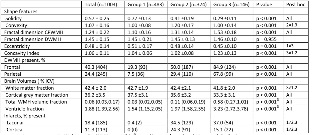
Brain imaging characteristics of the three groups are given in table 7. Groups are different in solidity, convexity, fractal dimension CPWMH, concavity index, eccentricity, number of DWMH (frontal, parietal, temporal and basal ganglia), WMF, GMF, VF, WMHF, lacunar and cortical infarct presence. On the other hand, fractal dimension of the DWMH and the number of occipital DWMH are not significantly different between groups.

Group 1 corresponding to patterns in the first clusters was characterized by the least brain atrophy (VF: 1.54(1.15,2.05), GMF: 37.5 ± 3.1), the lowest number infarcts (Lacunar: 0.4 %(2), Cortical: 0% (0)) and relatively small (WMHF: 0.03 (0.02,0.05)), solid and smooth (convexity: 1.00 ± 0.08, solidity: 0.77 ± 0.13, FD: 1.10 ± 0.16) CPWMH lesions. Group 2 is showing intermediate brain atrophy (VF: 1.97 (1.58,2.55), GMF: 35.6 ± 3.2), highest number of cortical infarcts (24.3 % (93)) and intermediate WMH volume (0.11(0.06,0.19)) with convex (convexity: 1.20 ± 0.17) CPWMH lesions. Group 3 has most brain atrophy (WMF: 41.8±2.0 vs. 42.7±1.9; p<0.001 & 42.4±2.1; p=0.006, GMF: 33.3±3.1, VF: 3.23 (2.72,3.78)) and the highest number of lacunar infarcts (37.0% (54)) and high WMH volume (3.23 (2.72,3.78)) with more irregular (concavity index: 1.23±0.13, FD: 1.53±0.18)) CPWMH lesions and less circular (0.45±0.10 vs. 0.51 ±0.17; p<0.001 & 0.48±0.14 ; p=0.08) DWMH lesions than group 1 and 2.

Between group differences in patient characteristics, vascular risk factors and primary disease location The clinical characteristics of the three groups are given in table 6. Significant differences were found in, mean age, sex, smoking, history of hypertension, diabetes, history of cerebral vascular disease, history of cardiac disease and history of an abdominal aneurysm were statistically different between groups. On the other hand, no significant differences were found in the body mass index, alcohol consumption,

hyperlipidaemia and history of peripheral vascular diseases.

Table 6. Demographics and clinical characteristics of the total cohort and clusters identified by cluster analysis.

Total (n=1003) Group 1 (n=483) Group 2 (n=374) Group 3 (n=146) P value Post hoc

Age (years) 59 ± 10 54 ± 9 61 ± 10 67 ± 7 p < 0.001 All

Gender, % men 79.1 (793) 79.7 (385) 75.9 (284) 84.9 (124) p = 0.07

Cardiovascular risk factors

BMI (kg/m2) 26.8 ± 3.8 26.8 ± 3.8 26.8 ± 3.9 26.4 ± 3.3 p = 0.441

Smoking (pack years) 22.4 ± 20.5 21.0 ± 19.6 22.6 ± 20.2 26.6 ± 23.6 p = 0.014 1≠3

Alcohol intake, current % 74.4 % (742) 76.0 (365) 72.0 (276) 75.3 (110) p = 0.694

Hypertension, % 51.6 (513) 43.4 (208) 59.8 (222) 57.2 (83) p < 0.001 1≠2,3

Hyperlipidaemia, % 79.6 (787) 81.6 (390) 77.0 (281) 79.5 (116) p = 0.259

Hyperhomocysteinemia, % 12.0 (120) 7.5 (36) 11.6 (43) 28.3 (41) p < 0.001 All

Diabetes mellitus, % 12.0 (120) 14.5 (69) 23.8 (87) 31.5 (45) p < 0.001 All

IMT (mm) 0.88 (0.73,1.05) 0.82 (0.70,0.97) 0.92 (0.77,1.08) 0.98 (0.87,1.15) p < 0.001Θ All

Vascular disease location, n (%)

Peripheral arterial disease 22.3 (224) 24.4 (118) 19.0 (71) 24.0 (35) p = 0.272

Cerebrovascular disease 22.7 (228) 8.1 (39) 36.6 (137) 35.6 (52) p < 0.001 1≠2,3

Coronary artery disease 57.7 (579) 64.6 (312) 53.2 (199) 46.6 (68) p < 0.001 1≠2,3

Abdominal aortic aneurysm 9.2 (92) 6.2 (30) 9.1 (34) 19.2 (28) p < 0.001 3≠1,2

Values are mean ± SD, % (n) or median (25, 75 percentile), Θ _{Natural log transformed to obtain normal distribution}

BMI: Body mass index, IMT: Intima-media thickness, all; all groups are significantly different

Table 7. Description of the total cohort and clusters identified by cluster analysis

Total (n=1003) Group 1 (n=483) Group 2 (n=374) Group 3 (n=146) P value Post hoc

Shape features

Solidity 0.57 ± 0.25 0.77 ±0.13 0.41 ±0.19 0.29 ±0.11 p < 0.001 All

Convexity 1.07 ± 0.16 1.00 ±0.08 1.20 ±0.17 1.00 ±0.14 p < 0.001 2≠1,3

Fractal dimension CPWMH 1.24 ± 0.22 1.10 ±0.16 1.31 ±0.14 1.53 ±0.18 p < 0.001 All

Fractal dimension DWMH 1.45 ± 0.15 1.45 ± 0.21 1.45 ± 0.13 1.46 ±0.10 p = 0.955

Eccentricity 0.48 ± 0.14 0.51 ± 0.17 0.48 ±0.14 0.45 ±0.10 p = 0.001 1≠3

Concavity Index 1.06 ± 0.11 1.04 ± 0.06 1.02 ±0.08 1.23 ±0.13 p < 0.001 3≠1,2

DWMH present, %

Frontal 40.3 (404) 19.3 (93) 50.0 (187) 84.9 (124) p < 0.001 All

Parietal 24.4 (245) 7.5 (36) 29.4 (110) 67.8 (99) p < 0.001 All

Brain Volumes ( % ICV)

White matter fraction 42.4 ± 2.0 42.7 ±1.9 42.4 ±2.1 41.8 ± 2.0 p < 0.001 3≠1,2

Cortical grey matter fraction 36.2 ±3.5 37.5 ±3.1 35.6 ±3.2 33.3 ± 3.1 p < 0.001 All

Total WMH volume fraction 0.06 (0.03,0.17) 0.03 (0.02,0.05) 0.11 (0.06,0.19) 0.58 (0.27,1.01) p < 0.001Θ All

Ventricle fraction 1.88 (1.39,2.56) 1.54 (1.15,2.05) 1.97 (1.58,2.55) 3.23 (2.72,3.78) p < 0.001Θ All

Infarcts, % present

Lacunar 18.4 (185) 0.4 (2) 34.5 (129) 37.0 (54) p < 0.001 1≠2,3

Cortical 11.3 (113) 0 (0) 24.3 (91) 15.1 (22) p < 0.001 1≠2,3

Values are mean ± SD, % (n) or median (25,75 percentile), Θ Natural log transformed to obtain normal distribution

Figure 11. Two CPWMH lesions (red) in two patients (A; 75 year old male, B; 59 year old male) are visualized with

corresponding convex hulls (blue) and calculated shape parameters. Both lesions have an approximately similar solidity (i.e. the ratio of the lesion volume to the convex hull volume), while lesion A has a higher convexity and fractal dimension compared to lesion B. The latter can be visually appreciated by the irregular aspect of lesion A compared to the relatively

smoother aspect of lesion B.

Table 8. Demographics and clinical characteristics of seven clusters identified by cluster analysis.

Group 1 Group 2 Group 3

P value Post hoc

Group A (n=300) Group B (n=183) Group C (n=49) Group D (n=120) Group E (n=205) Group F (n=118) Group G (n=28)

Age (years) 53±10 56±8 58±11 61±10 61±9 67±8 70±6 p < 0.001

A≠CDEFG, B≠DEFG, C≠AFG, D≠ABFG, E≠ABFG, F≠ABCDE , G≠ABCDE

Gender, % men 80.3 (241) 78.7 (144) 77.6 (38) 77.5 (93) 74.6 (153) 90.7 (107) 60.7 (17) p = 0.006 E≠F, F≠EG, G≠F; Smocking: A≠F; E≠F, F≠AE

Cardiovascular risk factors

BMI (kg/m2) 27.1±3.9 26.5±3.6 27.0±4.0 26.2±3.8 27.1±3.9 26.6±3.4 25.6±2.6 p = 0.106

Smoking (pack years) 19.6±18.8 23.3±20.5 22.9±18.5 25.5±22.6 20.8±18.8 27.9±23.5 22.4±20.5 p = 0.005

Alcohol intake, current % 74.5 (222) 78.6 (143) 83.7 (41) 68.3 (82) 71.3 (144) 76.3 (90) 71.4 (20) p = 0.165

Hypertension, % 45.5 (135) 40.1 (73) 61.2 (30) 64.2 (77) 56.9 (115) 54.7 (64) 67.9 (19) p < 0.001 A≠FG, C≠FG, E≠FG, B≠EFG, D≠G, F≠ABCE, G≠ABCDE

Hyperlipidaemia, % 82.9 (247) 79.4 (143) 72.9 (35) 74.8 (89) 79.3 (157) 79.7 (94) 78.6 (22) p = 0.541

Hyperhomocysteinemia, % 8 (24) 6.6 (12) 2.0 (1) 17.6 (21) 10.3 (21) 23.7 (28) 48.1 (13) p < 0.001 A≠FG, B≠EFG, C≠FG, D≠G, E≠FG, F≠ABCE, G≠ABCDE

Diabetes mellitus, % 16.2 (48) 11.7 (21) 18.8 (9) 24.6 (29) 24.5 (49) 33.0 (38) 25.0 (7) p < 0.001 A≠F, B≠F, F≠AB

IMT (mm) 0.83 (0.70,0.98) 0.82 (0.70,0.97) 0.96 (0.77,1.23) 0.93 (0.80,1.08) 0.92 (0.73,1.08) 1.00 (0.85,1.15) 0.97

(0.93,1.11) p < 0.001Θ A≠CDEFG, B≠CDEFG, C≠AB, D≠AB, E≠AB, F≠AB,

G≠AB

Vascular disease, n (%)

Peripheral arterial disease 23.3 (70) 26.2 (48) 14.3 (7) 13.3 (16) 23.4 (48) 26.3 (31) 14.3 (4) P=0.076

Cerebrovascular disease 9.0 (27) 6.6 (12) 77.6 (38) 55.8 (67) 15.6 (32) 31.4 (37) 53.6 (15) p < 0.001

A≠EDFG, B≠CDG, C≠ABEF, D≠ABEF, E≠ABFG, F≠ABCDE, G≠ABE

Coronary artery disease 63.7 (191) 66.1 (121) 32.7 (16) 38.3 (46) 66.8 (137) 50.8 (60) 28.6 (8) p < 0.001 A≠CDG, B≠CDG, C≠ABE, D≠ABE, E≠CDG, G≠ABE

Abdominal aortic aneurysm 5.3 (16) 7.7 (14) 0.0 (0) 14.2 (17) 8.3 (17) 18.6 (22) 21.4 (6) p < 0.001 A≠DFG, C≠FG, D≠A, F≠AC, G≠AC

Table 9. Description of the seven clusters identified by cluster analysis

Group 1 Group 2 Group 3

P value Post hoc

Group A (n=300) Group B (n=183) Group C (n=49) Group D (n=120) Group E (n=205) Group F (n=118) Group G (n=28) Shape features

Solidity 0.77±0.14 0.78±0.11 0.60±0.22 0.46±0.20 0.34±0.12 0.31±0.12 0.23±0.04 p < 0.001

A≠CDEFG, B≠CDEFG, C≠ all, D≠ all, E≠ABCDG, F≠ABCD, G≠ ABCDE

Convexity 0.99±0.09 1.00±0.06 1.07±0.14 1.13±0.13 1.28±0.15 1.04±0.11 0.81±0.11 p < 0.001

A≠CDEFG, B≠CDEFG, C≠ABDEG, D≠ all, E≠ all, F≠ ABDEG, G≠ all

Fractal dimension CPWMH 1.08±0.17 1.13±0.12 1.18±0.18 1.32±0.15 1.34±0.11 1.48±0.15 1.74±0.08 p < 0.001

A≠ all, B≠A DEFG, C≠ ADEFG, D≠ABCFG, E≠ABCFG, F≠ all, G≠all

Fractal dimension DWMH 1.45±0.23 1.45±0.17 1.42±0.16 1.45±0.14 1.46±0.11 1.46±0.11 1.44±0.06 P=0.860

Eccentricity 0.50±0.18 0.52±0.16 0.48±0.18 0.45±0.13 0.50±0.13 0.45±0.10 0.43±0.06 p < 0.001 B≠DF, D≠A, F≠B

Concavity Index 1.04±0.06 1.03±0.05 1.04±0.07 1.05±0.08 0.99±0.07 1.19±0.10 1.41±0.08 p < 0.001 A≠EFG, B≠EFG, C≠EFG, D≠EFG, E≠ all, F≠ all, G≠ all

DWMH present, % per lobe

Frontal 18.7 (56) 20.2 (37) 34.7 (17) 61.7 (74) 46.8 (96) 81.4 (96) 100.0 (28) p < 0.001

A≠ DEFG, B≠DEFG, C≠DFG, D≠ABCFG, E≠ABFG, F≠ ABCDE, G≠ ABCDE

Parietal 6.7 (20) 8.7 (16) 20.4 (10) 33.3 (40) 29.3 (60) 63.6 (75) 85.7 (24) p < 0.001

A≠ DEFG, B≠DEFG, C≠FG, D≠ABFG, E≠ABFG, F≠ ABCDE, G≠ ABCDE

Volume fraction (% ICV)

BPF 80.4 ± 2.5 79.7 ± 2.6 78.5 ±2.5 78.1 ± 2.9 78.7 ± 2.4 76.2 ± 2.8 76.6 ± 2.6 p < 0.001

A≠CDEFG, B≠CDEFG, C≠ABFG, D≠ABF, E≠ABFG, F≠ABCDE, G≠ABCE

WM 41.6±1.4 44.4±1.2 42.4±1.7 41.4±2.2 43.0±1.8 42.2±1.7 40.2±2.4 p < 0.001

A≠BCEFG, B≠ all, C≠ABDG, D≠BCEFF, E≠ABDFG, F≠ABDE, G≠ all

CGM 38.8±2.7 35.3±2.5 34.3±3.1 36.2±3.3 35.5±3.1 33.2±3.0 34.0±3.1 p < 0.001

A≠ all, B≠AF, C≠ AD, D≠ACFG, E≠ABCFG, F≠ABDE, G≠AD WMH 0.03 (0.01,0.05) 0.06 (0.03,0.17) 0.05 (0.03,0.09) 0.13 (0.06,0.22) 0.12 (0.07,0.19) 0.40 (0.23,0.75) 1.87

(1.51,2.38) p < 0.001Θ

A≠ all, B≠ all, C≠ all, D≠ ABCFG, E≠ABCFG, F≠ all, G≠ all Ventricle 1.48 (1.13,2.04) 1.88 (1.39,2.56) 1.91 (1.55,2.65) 2.17 (1.66,2.86) 1.92 (1.56,2.36) 3.24 (2.70,3.87) 3.08

(2.89,3.84) p < 0.001Θ

A≠CDEFG, B≠CDEFG, C≠ABFG, D≠ABFG, E≠ABFG, F≠ABCDE, G≠ABCDE

Infarcts, % present

Lacunar 0.0 (0) 1.1 (2) 8.2 (4) 95.8 (115) 4.9 (10) 29.7 (35) 67.9 (19) p < 0.001

A≠CDEFG, B≠DFG, C≠ADG, D≠ all, E≠ADFG, F≠ABDEG, G≠ all

Cortical 0.0 (0) 0.0 (0) 100.0 (49) 32.5 (39) 1.5 (3) 11.0 (13) 32.1 (9) p < 0.001

A≠ CDEFG, B≠ CDFG, C≠ all, D≠ABCEF, E≠DFG, F≠ ABCDE, G≠ABCE

Values are mean ± SD, % (n) or median (25,75 percentile), Θ Natural log transformed to obtain normal distribution

Seven subgroup approach

The obtained dendogram was cut to produce seven distinct clusters of brain imaging features (figure 11) within this cohort of patients with manifest arterial disease. Cluster A grouped 300 patients (30%), cluster B: 49 (5%), cluster C: 120 (12%), cluster D: 28 (3%), cluster E: 205 (20%), cluster F: 118 (12%) and the final cluster (F) grouped 183 patients (18%).

Brain imaging characteristics of the seven groups are given in table 9. Groups are distinguished based on solidity, convexity, fractal dimension CPWMH, concavity index, eccentricity, number of DWMH (frontal, parietal, occipital, temporal and basal ganglia), WMF, GMF, VF, WMHF, lacunar and cortical infarct presence. On the other hand, the fractal dimension of the DWMH is not significantly different between any groups.

The clinical characteristics of the seven groups are given in table 8. Significant differences were found in, mean age, sex, alcohol consumption, smoking, history of hypertension, diabetes, history of cerebral vascular disease, history of cardiac disease and history of an abdominal aneurysm were statistically different between groups. On the other hand, no significant differences were found in the body mass index, hyperlipidaemia and history of peripheral vascular diseases.

Group A and B have relatively few brain abnormalities and are only significantly different from each other in FD of the CPWMH, WM volume, GM volume and WMH volume. Where group A has a high CGM volume and group B has a high WM volume. These groups are characterized by the least amount of brain atrophy, the lowest number of infarcts (similar to group E) and have relative small (WMH volume:

0.03(0.01,0.05);p<0.05*BCDEFG & 0.06(0.03,0.17);p<0.05*ACDEFG), solid (solidity: 0.77±0.14;p<0.05*CDEFG & 0.78±0.11;p<0.05*CDEFG) and smooth (convexity: 0.99±0.09;p<0.05*CDEFG & 1.00±0.06;p<0.05*CDEFG, FD: 1.08±0.17;p<0.05 & 1.13±0.12;p<0.05*ADEFG) CPWMH lesions. Additionally, group B has the most round DWMH lesions (eccentricity: 0.52±0.16;p<0.05*DF).

Group A and B are the youngest groups (age: 53±10;p<0.05*CDEFG & 56±8;p<0.05*DEFG) with the least smokers in group A (pack years: 19.6±18.8;p<0.05*F), relative few people with hypertension (45.5(135);p<0.05*D & 40.1(73);p<0.05*DE), diabetes (16.2(48);p<0.05*F & 11.7(21);p<0.05*F) and hyperhomocysteinemia (8.0(24);p<0.05*FG & 6.6(24);p<0.05*EFG). These groups also has a relative small IMT (0.83(0.70,0.98);p<0.05*CDEFG & 0.82(0.70,0.98);p<0.05*CDEFG) and few patients with a history of AAA (5.3(16);p<0.05*DFG & 7.7(14)), cerebrovascular disease (9.0(27);p<0.05*CDFG & 6.6(12);p<0.05*CDG) and many patients have coronary artery disease (63.7(191);p<0.05*CDG & 66.1(121);p<0.05*CDG).

Group C can be considered a large vessel disease group characterized by a small (0.05(0.03,0.09);p<0.05), solid (solidity: 0.60±0.22;p<0.05) and smooth WMH (FD of the CPWMH:1.18±0.18;p<0.05*ADEFG,

convexity:1.07±0.14;p<0.05*ADEFG), intermediate brain atrophy (BPF: 78.5±2.5;p<0.05*AFG), few lacunar infarcts (8.2% (4);p<0.05*ADG) and many cortical infarcts (100% (49) );p<0.05). This group, has an intermediate age (58±11;p<0.05*AFG), relative high number of patients with hypertension (61.2(30)) and few patients with hyperhomocysteinemia (2.0(1);p<0.05*FG). Furthermore, this group has a relative large IMT (0.96(0.77,1.23;p<0.05*AB)) especially for these relative young patients. Many patients in this group suffer from cerebrovascular disease (77.6(38);p<0.05ABEF) and few suffer from coronary artery disease (32.7(16);p<0.05*ABE) or AAA (0.0(0);p<0.05*DG).

Group D can be considered a lacunar infarct group characterized by WMH with an intermediate volume (0.13(0.06,0.22);p<0.05*ABCFD) with increased roughness of the CPWMH lesions compared to group C (FD: 1.32±0.15;p<0.05*ABCFG, solidity: 0.46±0.20;p<0.05), intermediate brain atrophy (BPF: 78.1±2.9;p<0.05*ABF), cortical infarct presence (32.5%(39) );p<0.05*ABCEF and many lacunar infarcts (95.7%(115) );p<0.05) and relatively elongated DWMH lesions comparable to group F (0.45±0.13;p<0.05*B). This group, has an intermediate age (61±10;p<0.05*ABFG) with relatively heavy smokers (pack years: 25.5±22.6), relative high number of patients with hypertension (64.2(77)) and hyperhomocysteinemia (17.6(21);p<0.05*G). This group has a relative large IMT (0.96(0.77,1.23;p<0.05*AB)) and many patients in this group have

cerebrovascular disease (55.8(67);p<0.05ABEF) and AAA (14.2(17);p<0.05*A) and few have coronary artery disease (32.7(16);p<0.05*ABE).

Group E is characterized by more elongated CPWMH around the ventricles (solidity:

0.34±0.12;p<0.05*ABCDG, convexity: 1.28±0.15;p<0.05, FD: 1.34±0.11;p<0.05*ABCFG), relative few frontal DWMH lesions compared to group D with the same volume (46.8%(96) vs. 61.7%(74)), an intermediate amount of brain atrophy (BPF: 78.7±2.4;p<0.05*ABFG) and few infarcts (LI: 4.9%(10);p<0.05*ADFG,

of patients with hypertension (56.9(115);p<0.05*B) and few patients with hyperhomocysteinemia (10.3(21);p<0.05*FG). This group has a relative large IMT (0.93(0.80,1.08;p<0.05*AB)) and few patients in this group have cerebrovascular disease (15.6(32);p<0.05ABFG) and many have coronary artery disease (66.8(137);p<0.05*CDG).

Group F is characterized by an intermediate burden of WMH (0.40(0.23,0.75);p<0.05) with more irregular CPWMH lesions (solidity: 0.31±0.12;p<0.05*ABCDG, FD: 1.48±0.15;p<0.05*ABCDFG and concavity Index: 1.19±0.10;p<0.05*ABCDFG) and cerebral atrophy (BPF: 76.2±2.8;p<0.05*ABCDE). This group has a moderate number of infarcts (LI: 29.7%(35) ;p<0.05*ABDEG, CI:11.0%(13) ;p<0.05*ABCDE). This group represents older individuals of this cohort (age: 67±8;p<0.05*ABCDE) with the heaviest smokers (pack years:

27.9±23.5;p<0.05*A) and relatively many patients with hyperhomocysteinemia (23.7(28);p<0.05*ABCE), diabetes mellitus (33.0(38);p<0.05*AB) and a history of AAA (18.6(22);p<0.05*AC) and an intermediate number of patients with cerebrovascular disease (31.4(37);p<0.05*ABCDE).

Group G can be considered a group of older individuals with SVD and is characterized by the highest burden of WMH (1.87(1.51,2.38);p<0.05), these lesions have the highest textural roughness (solidity: 0.23±0.04;p<0.05*ABCDE, convexity: 0.81±0.11;p<0.05, FD:1.74±0.08;p<0.05), highest number and most elongated DWMH (eccentricity: 0.43±0.06), a relative large amount of cerebral atrophy (BPF:

76.6±2.6;p<0.05*ABCE) a high prevalence of lacunar infarcts (LI: 67.9%(19) ;p<0.05, CI:32.1%(9)

;p<0.05*ABCE). This group of older individuals with SVD (age: 70±6;p<0.05*ABCDE) has the most patients with hypertension (67.9(19)) and hyperhomocysteinemia (48.1(13);p<0.05*ABCDE). History of cerebrovascular (53.6(15);p<0.05*ABE) and AAA (21.4(6);p<0.05*AC) are common and few patients have a history of coronary artery disease (28.6(22);p<0.05*ABE).

Figure 12. The chance of WMH and BPF presence per cluster in the three cluster approach. Probability of WMH increases with cluster number (A). Highest probability of WMH occurs at the anterior horns (caps) and body (bands) of the lateral ventricles. An increase in atrophy with an increased lateral ventricle size can be observed with increasing cluster number (B).