OF
C
OFFEEJesús G. Otero Department of Economics
University of Warwick and
Costas Milas Department of Economics
University of Warwick
December 1998
ABSTRACT
1. Introduction
The international price movements of primary products has been the subject of extensive research in developing countries. Primary products, unlike manufactures, usually have low supply and demand price elasticities (in absolute value), so that a given shift in one of the curves causes a much larger change in prices, than if the elasticities are larger in absolute value.1 Moreover, these price fluctuations tend to have important effects on developing countries, since they are still largely dependent on primary-commodity markets for their principal export earnings, and the relative importance of the commodity sector in these countries is much greater than in most developed countries.2
Coffee constitutes one of the most important export products in developing countries. It is difficult to speak of an international market for coffee in the strict sense of the term, since there are a number of coffee varieties that can be distinguished, such as Unwashed Arabicas (mainly coffee from Brazil), Colombian Mild Arabicas (mainly coffee from Colombia), Other Mild Arabicas (mainly coffee from other Latin American countries), and Robusta (mainly coffee from African countries and Southeast Asia).3 The formation of the coffee price in the world market can be explained by several factors, including changes in aggregate demand or supply, the quality of the product, the country of origin, the trading market, and the existence or non existence of export quota systems.
1
Adams and Behrman (1982), for example, find a strong association between price inelasticities and price instabilities for a number of primary commodities.
2
In 1991, for instance, the share of fuels, minerals, metals, and other primary commodities in the exports of low- and middle-income countries amounted to over 50%, compared with a world share of approximately 25% (these figures are from the World Bank 1993).
3
Vogelvang (1992) has investigated the existence of long-run relationships between the spot prices of the four main types of coffee discussed above, as originated from trade in the New York market. Using quarterly data over the period 1960(1)-1982(3), Vogelvang found evidence of two long-run equilibrium relationships: one involving Other Milds and Colombian Milds, and the other one involving Robusta coffee, Other Milds and Colombian Milds. Since 1982, however, the world price of these types of coffee has exhibited substantial variations, such as the sharp increases of 1985-86, 1994-95 and 1997, mainly due to adverse weather conditions in Brazil (the world’s largest coffee producer), and the severe price fall of 1992-93 originated from a situation of excess supply.
Drawing on the earlier work by Vogelvang (1992), this paper re-examines the validity of the cointegrating properties of the four coffee price series, extending the sample period up to the second quarter of 1998 in order to account for the events that have occurred in the coffee market during the last fifteen years. In addition to that, we examine the persistence profile properties of the estimated cointegrating vectors (see Pesaran and Shin, 1996). Persistence profile analysis constitutes a useful visual tool to investigate the speed with which deviations from the estimated long-run cointegrating relations, resulting from system-wide shocks, are eliminated. Out of sample forecasting analysis serves as a guide to test the ability of the estimated model to capture future coffee price movements in the world market.
Milds and Colombian Milds is no longer supported by the data. Instead, cointegration analysis supports a long-run relationship between the prices of Unwashed Arabicas and Robusta coffee.
The paper is organised as follows. Section 2 applies multivariate cointegration analysis to determine the existence of long-run equilibrium relationships between the prices of the four coffee varieties. Section 3 presents the short-run dynamics of the empirical model and discusses its forecasting performance. Section 4 offers some concluding remarks.
2. The empirical model: Long-run behaviour
Our model uses a set of p = 4 endogenous variables, y =[PUA, POM, PROB, PCOL]′, where PUA, POM, PROB and PCOL refer to the spot prices of Unwashed Arabicas, Other Milds, Robusta, and Colombian coffees in the New York market, respectively.4 The data are quarterly observations from 1962(1) to 1998(2), although the model is estimated until 1993(4) leaving the last four and a half years to evaluate its forecasting performance. All the variables are in logarithms.
Following Johansen (1988, 1995), we write a p-dimensional Vector Error Correction Model (VECM) as:
T t y y y t k i t i t i
t , 1,...,
1
1
1 +µ+ε =
Π + ∆ Γ = ∆
∑
− = − − (1)where ∆ is the first difference operator, yt is the set of I(1) stochastic variables
discussed above, εt ~niid( , )0 Σ , µ is a drift parameter, and Π is a (p x p) matrix of
4
the form Π =αβ′, where α and β are both (p x r) matrices of full rank, with β
containing the r cointegrating relationships and α carrying the corresponding loadings
in each of the r vectors.
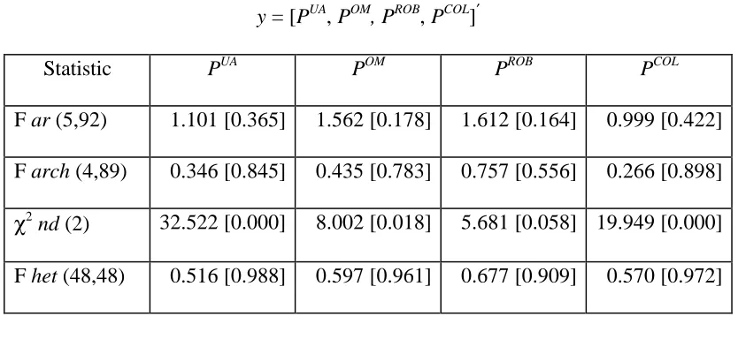
Preliminary analysis of the statistical properties of the data using the Augmented Dickey-Fuller (ADF) tests suggested that all series are I(1) without drift when considered in levels, and I(0) in first differences.5 The first panel of Table I reports the diagnostic tests for the levels of the four equations in (1), using a lag length of k = 6 (k was selected using the Akaike information criterion), and allowing for the intercept
term (i.e. µ) to enter the cointegrating space, since the series have a zero drift term. The diagnostic tests show no problems of residual serial correlation, ARCH effects and heteroscedasticity; however normality fails in the equations for PUA, POM and PCOL. The normality failure may be the result of several exogenous shocks to the coffee price series during the sample period, so that there is also the need to include some intervention dummy variables to account for the corresponding short-run effects. The most important of these shocks refer to adverse weather conditions in Brazil, and the collapse of the international coffee agreement in 1989, following opposition by the United States and some other consuming countries.6 The second panel of Table I shows the diagnostic tests of the VAR model including the intervention dummies; as can be seen, the normality tests improve substantially;
5
The presence of a unit root in the price series is also confirmed by the Phillips-Perron tests, and by the visual inspection of the correlograms of the series. A detailed Appendix on these tests is available from the authors upon request.
6
however in the equation for PUA the normality test is still significant at the one per cent level.
Table I. Diagnostic statistics y =[PUA, POM, PROB, PCOL]′
Statistic PUA POM PROB PCOL
F ar (5,92) 1.101 [0.365] 1.562 [0.178] 1.612 [0.164] 0.999 [0.422]
F arch (4,89) 0.346 [0.845] 0.435 [0.783] 0.757 [0.556] 0.266 [0.898]
χ2
nd (2) 32.522 [0.000] 8.002 [0.018] 5.681 [0.058] 19.949 [0.000]
F het (48,48) 0.516 [0.988] 0.597 [0.961] 0.677 [0.909] 0.570 [0.972]
y =[PUA, POM, PROB, PCOL]′ with intervention dummies
Statistic PUA POM PROB PCOL
F ar (5,90) 0.908[0.479] 0.882[0.496] 0.914[0.475] 0.792[0.558] F arch (4,87) 1.458[0.221] 2.441[0.052] 2.107[0.086] 1.281[0.283]
χ2
nd (2) 9.756[0.007] 3.681[0.158] 6.611[0.036] 7.186[0.027]
F het (48,46) 1.456[0.101] 1.124[0.345] 1.064[0.416] 1.132[0.337]
Notes: F ar is the Lagrange Multiplier F-test for residual serial correlation of up to fifth order. F arch is the fourth order Autoregressive Conditional Heteroscedasticity F-test. χ2 nd is a Chi-square test for normality. F het is an F test for heteroscedasticity. Numbers in parentheses indicate the degrees of freedom of the test statistics. Numbers in square brackets are the probability values of the test statistics.
The determination of the number of cointegrating vectors is based on the
maximal eigenvalue (λ-max) and the trace (λ-trace) tests. Allowing for short-run effects from the intervention dummies, cointegration results are shown in Table II, which reports the λi eigenvalues, the λ-max and the trace statistics, and the 95% and 90%
but there is evidence of at least one vector at the 90% level. The trace statistic supports the existence of r = 2 cointegrating vectors at the 95% level. Given that the trace statistic seems to be more robust to normality failures (see Cheung and Lai, 1993), we move on by assuming the existence of two cointegrating vectors, which are reported in Table III along with their corresponding adjustment coefficients.7
Table II. Eigenvalues, test statistics, and critical values
λi λ-max λ-trace
H0 H1 Stat. 95% 90% H0 H1 Stat. 95% 90%
0.194 r = 0 r = 1 26.26 28.14 25.56 r = 0 r≥ 1 61.99 53.12 49.65
0.149 r≤ 1 r = 2 19.68 22.00 19.77 r≤ 1 r≥ 2 35.73 34.91 32.00 0.079 r≤ 2 r = 3 10.06 15.67 13.75 r≤ 2 r≥ 3 16.05 19.96 17.85
0.048 r≤ 3 r = 4 5.99 9.24 7.52 r≤ 3 r = 4 5.99 9.24 7.52
Notes: r denotes the number of cointegration vectors. The critical values of the λ-max and λ-trace statistics are taken from Osterwald-Lenum (1992).
7
Table III. Estimated cointegrating vectors (β) and weights (α)
β1 β2 α1 α2
PUA 1.000 0.338 -0.301 -0.736
POM -0.429 1.000 0.074 -0.755
PROB -0.665 -0.161 0.216 -0.695
PCOL 0.052 -1.156 -0.026 -0.504
µ 0.010 -0.031 -
-The next step involves the identification of the two cointegrating vectors. In a recent paper, Pesaran and Shin (1995) develop a long-run structural modelling framework for identification and hypothesis testing in cointegrating systems. According to this
approach, exact identification of β (in Π = αβ′) requires at least r restrictions (including the normalising restrictions) on each of the r cointegrating relationships. These exactly identifying restrictions do not impose any testable restrictions on the cointegrating VAR model. It is only the validity of additional over-identifying restrictions that can be tested using standard Likelihood Ratio tests. Under the assumption of r = 2 cointegrating relationships, we need to impose two restrictions on each of the two vectors to exactly identify them. To do so, we denote the two vectors associated with y =[PUA, POM, PROB,
PCOL, µ]′, by:
β1 = [β11, β12, β13, β14, β15]′,
and
β2 = [β21, β22, β23, β24, β25]′,
term, µ, respectively. We view the first vector as a coffee price equation for Unwashed Arabicas (i.e. PUA), and the second one as a coffee price equation for Other Milds (i.e. POM), and impose the following exactly identifying restrictions:
β11 = 1, β14 = 0 (on the first vector),
and
β22 = 1, β23 = 0, (on the second vector).
The set of non-testable restrictions on β1, refers to normalisation with respect to
the price of Unwashed Arabicas (i.e. β11 = 1) and long-run exclusion of the price of
Colombian coffee (i.e. β14 = 0), as supported by the unrestricted estimates of the first
vector (see Table III). The set of non-testable restrictions on β2, refers to normalisation
with respect to the coffee price of Other Milds (i.e. β22 = 1) and long-run exclusion of the
price of Robusta coffee (i.e. β23 = 0), since the latter estimate is rather small in the second cointegrating vector. Having imposed exactly identifying restrictions on the two vectors, we then test the validity of further over-identifying restrictions:
β13 = -1, β12 = 0 (on the first vector),
and
β24 = -1, β21 = 0 (on the second vector).
The two testable over-identifying restrictions on the first vector refer to proportionality with negative sign between the price of Unwashed Arabicas and the price
of Robusta coffee (i.e. β13 = -1), and long-run exclusion of the price of Other Milds (i.e.
β12 = 0). The two testable over-identifying restrictions on the second vector refer to
proportionality with negative sign between the prices of Other Milds and Colombian
coffee (i.e. β24 = -1), and long-run exclusion of the price of Unwashed Arabicas (i.e.
two restrictions on the first cointegrating vector and two restrictions on the second one. The Likelihood Ratio test statistic for testing all four over-identifying restrictions is
distributed as a χ2(4) under the null hypothesis, giving a value of 5.868 which is insignificant at the 5% level (p-value = 0.209). Imposing the restrictions discussed above, yields the following restricted cointegrating vectors:
PUA = PROB + 0.241 (0.021) and
POM = PCOL− 0.091 (0.010),
where standard errors are given in parentheses next to the estimated coefficients. The first cointegrating vector is interpreted as a long-run equilibrium relation between the prices of Unwashed Arabicas and Robusta coffee, with the estimated positive intercept supporting the price differential that has historically characterised these two types of coffee.8 The estimates of the adjustment coefficients on PUA, POM, PROB and PCOL are equal to -0.364, -0.153, 0.024 and -0.167, respectively. The second cointegrating vector is interpreted as a long-run equilibrium equation between the prices of Other Milds and Colombian coffee, both of which are Arabica coffees; the estimated negative intercept can be thought of as a quality premium of the Colombian coffee over Other Milds, a result that is consistent with historical evidence.9 In the second vector, the estimates of the adjustment coefficients on PUA, POM,PROB and PCOL are equal to -0.451, -0.793, -0.671 and -0.424, respectively.
It is worth mentioning that our finding of a long-run equilibrium relationship between POM and PCOL is in accordance with Vogelvang (1992). However, the developments in the coffee market since the early 1980s, no longer support a long-run
8
Arabicas coffees are considered of better quality than Robustas. See Junguito and Pizano (1993, Chapter 4) for an analysis of the price differentials between the main coffee varieties.
9
equilibrium relationship among PROB, POM and PCOL; rather, we find evidence of a cointegrating vector between PUAand PROBalone.
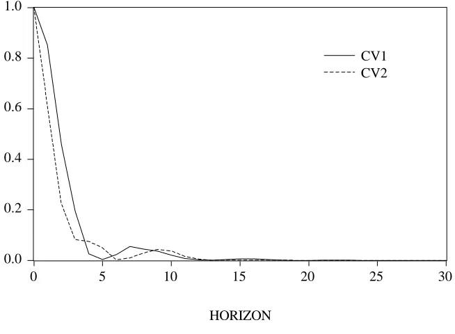
Having identified the two cointegrating relationships we proceed by plotting their persistent profiles. The persistent profile analysis (see e.g. Pesaran and Shin, 1996), sheds some light on the speed of convergence of the two estimated vectors towards their long-run equilibrium following system-wide shocks. This analysis thus provides complementary evidence that the estimated vectors are indeed cointegrating relationships. Furthermore, Pesaran and Shin (1996) show that the persistent profile approach has the advantage of being invariant to the way shocks in the underlying VAR model are orthogonalised, and therefore provides an important extension to the traditional impulse response analysis, which is sensitive to the ordering of the variables in the VAR (see e.g. Lütkepohl, 1991).
Figure 1 shows the persistence profiles for the estimated cointegrating relations following system-wide shocks.10 As can be seen from the figure, the estimated persistence profiles of both equations converge to zero reasonably quickly. Indeed, the persistence profile of the two cointegrating vectors show that almost full adjustment is completed within a year. The fact that shocks have short-lived effects on the cointegrating relations, is an indication that the markets for the various types of coffee are closely related and that economic forces act rapidly; hence, short-run discrepancies in the equilibrium relationships do not grow systematically over time.
10
Figure 1. Persistence profiles of cointegrating vectors to system-wide shocks
0.0 0.2 0.4 0.6 0.8 1.0
0 5 10 15 20 25 30
HORIZON
CV1 CV2
Note: CV1 = PUA - PROB - 0.241, and CV2 = POM - PCOL + 0.091.
3. Short-run dynamics and forecasting performance of the model
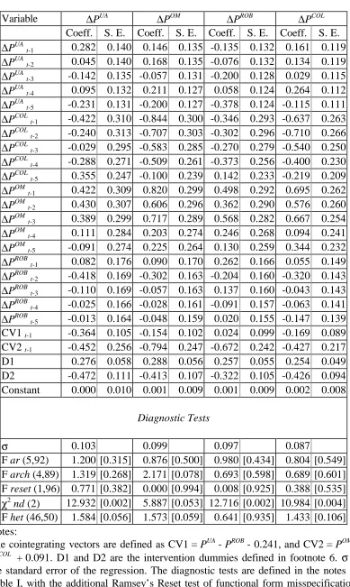
Once we have found evidence of long-run equilibrium relationships among the coffee price series, we estimate the VAR model in error correction form. The lag length in the
equations for ∆PUA, ∆POM, ∆PROB and ∆PCOL is equal to five, since we included six lags in the VAR model of the variables in levels. Ordinary least squares estimates of the reduced form error correction models are reported in Table IV, along with their corresponding standard errors and diagnostic tests. All equations pass the LM test for residual serial correlation of up to fifth order, Engle’s LM[4] test for ARCH, Ramsey’s RESET test, and White’s test for heteroscedasticity. Nonetheless, the test for normality is significant at the
one per cent level in the equations for ∆PUA, ∆PROB and ∆PCOL.
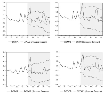
that is, ∆PUA, ∆POM, ∆PROB and ∆PCOL. The dynamic solution of the model begins in 1994(1), continuing as long as historical data of the coffee price series are available, that is, 1998(2). Dynamic solution performs multi-step forecasts, using historical data for lagged endogenous variables if they are dated prior to the first period of the simulation; thereafter it uses the values forecasted by the model itself. Hence, the simulation corresponds to a dynamic “ex-ante” forecast, which allows us to assess the ability of the model to predict beyond the estimation period.
Figure 2 plots the sequence of dynamic forecasts with error bars for 95 per cent confidence intervals.11 As can be seen, there is not much increase in uncertainty for the four equations in first differences, and the actual values of the series lie within their confidence intervals, with the notable exception of 1994(3) and 1997(2). The inability of the model to capture the large movements of the coffee prices over these periods can be explained by exogenous shocks to the system, notably adverse weather conditions. Indeed, between the second and third quarter of 1994, world coffee prices increased approximately by 80%, following news of two frosts in the coffee-producing areas of Brazil over the June-July period. Furthermore, during the first half of 1997, the prices of the three Arabica coffees increased sharply by some 90%, following three consecutive years of low crops in Brazil, Colombia and other major coffee producing countries.12 At the same time, Robusta prices increased less (around 30%), due to good crops in Vietnam and Uganda.
11
These dynamic forecasts are equivalent to 18-step ahead forecasts (i.e. 1994(1) to 1998(2)). The forecasting analysis was performed using PcFiml 9.0 (see Hendry and Doornik, 1997).
12
Table IV. Error correction model
Variable ∆PUA ∆POM ∆PROB ∆PCOL
Coeff. S. E. Coeff. S. E. Coeff. S. E. Coeff. S. E.
∆PUAt-1 0.282 0.140 0.146 0.135 -0.135 0.132 0.161 0.119
∆PUAt-2 0.045 0.140 0.168 0.135 -0.076 0.132 0.134 0.119
∆PUAt-3 -0.142 0.135 -0.057 0.131 -0.200 0.128 0.029 0.115
∆PUAt-4 0.095 0.132 0.211 0.127 0.058 0.124 0.264 0.112
∆PUAt-5 -0.231 0.131 -0.200 0.127 -0.378 0.124 -0.115 0.111
∆PCOLt-1 -0.422 0.310 -0.844 0.300 -0.346 0.293 -0.637 0.263
∆PCOLt-2 -0.240 0.313 -0.707 0.303 -0.302 0.296 -0.710 0.266
∆PCOLt-3 -0.029 0.295 -0.583 0.285 -0.270 0.279 -0.540 0.250
∆PCOLt-4 -0.288 0.271 -0.509 0.261 -0.373 0.256 -0.400 0.230
∆PCOLt-5 0.355 0.247 -0.100 0.239 0.142 0.233 -0.219 0.209
∆POMt-1 0.422 0.309 0.820 0.299 0.498 0.292 0.695 0.262
∆POMt-2 0.430 0.307 0.606 0.296 0.362 0.290 0.576 0.260
∆POMt-3 0.389 0.299 0.717 0.289 0.568 0.282 0.667 0.254
∆POMt-4 0.111 0.284 0.203 0.274 0.246 0.268 0.094 0.241
∆POMt-5 -0.091 0.274 0.225 0.264 0.130 0.259 0.344 0.232
∆PROBt-1 0.082 0.176 0.090 0.170 0.262 0.166 0.055 0.149
∆PROBt-2 -0.418 0.169 -0.302 0.163 -0.204 0.160 -0.320 0.143
∆PROBt-3 -0.110 0.169 -0.057 0.163 0.137 0.160 -0.043 0.143
∆PROBt-4 -0.025 0.166 -0.028 0.161 -0.091 0.157 -0.063 0.141
∆PROBt-5 -0.013 0.164 -0.048 0.159 0.020 0.155 -0.147 0.139 CV1 t-1 -0.364 0.105 -0.154 0.102 0.024 0.099 -0.169 0.089 CV2 t-1 -0.452 0.256 -0.794 0.247 -0.672 0.242 -0.427 0.217 D1 0.276 0.058 0.288 0.056 0.257 0.055 0.254 0.049 D2 -0.472 0.111 -0.413 0.107 -0.322 0.105 -0.426 0.094 Constant 0.000 0.010 0.001 0.009 0.001 0.009 0.002 0.008
Diagnostic Tests
σ 0.103 0.099 0.097 0.087
F ar (5,92) 1.200 [0.315] 0.876 [0.500] 0.980 [0.434] 0.804 [0.549] F arch (4,89) 1.319 [0.268] 2.171 [0.078] 0.693 [0.598] 0.689 [0.601] F reset (1,96) 0.771 [0.382] 0.000 [0.994] 0.008 [0.925] 0.388 [0.535]
χ2
nd (2) 12.932 [0.002] 5.887 [0.053] 12.716 [0.002] 10.984 [0.004] F het (46,50) 1.584 [0.056] 1.573 [0.059] 0.641 [0.935] 1.433 [0.106] Notes:
Figure 2. Dynamic forecasts -0.8 -0.6 -0.4 -0.2 0.0 0.2 0.4 0.6 0.8
90 91 92 93 94 95 96 97 98
DPUA DPUA (dynamic forecast)
-0.8 -0.6 -0.4 -0.2 0.0 0.2 0.4 0.6
90 91 92 93 94 95 96 97 98
DPOM DPOM (dynamic forecast)
-0.6 -0.4 -0.2 0.0 0.2 0.4 0.6 0.8
90 91 92 93 94 95 96 97 98
DPROB DPROB (dynamic forecast)
-0.8 -0.6 -0.4 -0.2 0.0 0.2 0.4 0.6
90 91 92 93 94 95 96 97 98
4. Concluding remarks
In this paper we have investigated long-run relationships among the spot prices of four main varieties of coffee: Unwashed Arabicas, Colombian Mild Arabicas, Other Mild Arabicas, and Robusta. Historically, the prices of these types of coffee have exhibited similarities in their behaviour, and so it is interesting to examine the way in which they are related to each other.
Using quarterly data from 1962(1) to 1993(4), we identified two long-run equilibrium relationships: one between the prices of Other Milds and Colombian coffee, and the other one between the prices of Unwashed Arabicas and Robusta coffee. Our results partially confirmed previous findings by Vogelvang (1992), who, using a shorter sample period, found evidence supporting the first cointegrating relation but not the second one.
References
Adams, G. and J. Behrman (1982). Commodity Exports and Economic Development: the Commodity Problem and Policy in Developing Countries, Lexington Books, Massachusetts.
Cheung, Y.W. and K.S. Lai (1993). ‘Finite-sample sizes of Johansen’s likelihood ratio tests for cointegration’, Oxford Bulletin of Economics and Statistics, 55, 313-328. Hendry, D.F. and J.A. Doornik (1997). Modelling Dynamic Systems Using PcFiml
9.0 for Windows, International Thomson Business Press.
Johansen, S. (1988). ‘Statistical analysis of cointegration vectors’, Journal of Economic Dynamics and Control, 12, 231-254.
Johansen, S. (1995). Likelihood-based Inference in Cointegrated Vector Autoregressive Models, Oxford University Press, Oxford.
Junguito, R. and D. Pizano (1993). El Comercio Exterior y la Política Internacional del Café. Fondo Cultural Cafetero – Fedesarrollo, Bogota.
Lütkepohl H. (1991). Introduction to Multiple Time Series Analysis, Springer-Verlag, New York.
Osterwald-Lenum, M. (1992). ‘A note with quantiles of the asymptotic distribution of the maximum likelihood cointegration rank test statistics’, Oxford Bulletin of Economics and Statistics, 54, 461-472.
Pesaran, M.H. and B. Pesaran (1997). Microfit 4.0: An Interactive Econometric Software Package, Oxford University Press, Oxford.
Pesaran, M.H. and Y.S. Shin (1996). ‘Cointegration and speed of convergence to equilibrium’, Journal of Econometrics, 71, 117-143.
Vogelvang, E. (1992). ‘Hypothesis testing concerning relationships between spot prices of various types of coffee’, Journal of Applied Econometrics, 7, 191-201. World Bank (1993). World Development Report, Oxford University Press, Oxford. World Bank. ‘Commodity Markets and the Developing Countries’. A World Bank