NRU-HSE at SemEval-2016 Task 4: Comparative Analysis of Two Iterative Methods Using
Quantification Library
Nikolay Karpov, Alexander Porshnev, Kirill Rudakov
National Research University Higher School of Economics
25/12 Bolshaja Pecherskaja str. 603155
Nizhny Novgorod, Russia
{
nkarpov
, aporshnev}@hse.ru,
[email protected]
Abstract
In many areas, such as social science, politics or
market research, people need to track sentiment
and their changes over time. For sentiment analysis
in this field it is more important to correctly
esti-mate proportions of each sentiment expressed in
the set of documents (quantification task) than to
accurately estimate sentiment of a particular
doc-ument (classification). Basically, our study was
aimed to analyze the effectiveness of two iterative
quantification techniques and to compare their
ef-fectiveness with baseline methods. All the
tech-niques are evaluated using a set of synthesized data
and the SemEval-2016 Task4 dataset. We made the
quantification methods from this paper available as
a Python open source library. The results of
com-parison and possible limitations of the
quantifica-tion techniques are discussed.
1
IntroductionIn many areas, such as customer-relationship manage-ment or opinion mining, people need to track changes over time and measure proportions of documents ex-pressing different sentiments. In these situations, the task of accurate categorization of each document is re-placed by the task of providing accurate proportions of documents from each class (quantification). George Forman suggested defining the ‘quantification task’ as finding the best estimate for the amount of cases in each class in a test set, using a training set with substantially different class distribution (Forman, 2008).
Application of the quantification approach in opinion mining (Esuli et al., 2010), network-behavior analysis (Tang et al., 2010), word-sense disambiguation (Chan and Ng, 2006), remote sensing (Guerrero-Curieses et al., 2009), quality control (Sánchez et al., 2008), moni-toring support-call logs (Forman et al., 2006) and credit
scoring (Hand and others, 2006) showed high perfor-mance even with a relatively small training set.
Although quantification techniques are able to pro-vide accurate sentiment analysis of proportions in situa-tions of distribution drift, the question of optimal tech-nique for analysis of tweets still raises a lot of questions. It is worth mentioning that sentiment analysis of tweets presents additional challenges to natural language pro-cessing, because of the small amount of text (less than 140 characters in each document), usage of creative spelling (e.g. “happpyyy”, “some1 yg bner2 tulus”), ab-breviations (such as “wth” or “lol”), informal construc-tions (“hahahaha yava quiet so !ma I m bored av even home nw”) and hashtags (BREAKING: US GDP growth is back! #kidding), which are a type of tagging for Twitter messages.
In our paper we used several quantification methods mentioned in literature as the best ones and evaluated them by comparing their effectiveness with one another and with baseline methods.
The paper is organized as follows. In Section 2, we first look at the notation, then we briefly overview six methods to solve the quantification problem. Section 3 describes two datasets we use in our research. Section 4 describes the results of our experiments, while Section 5 concludes the work defining open research issues for further investigation.
2
Quantification MethodsIn this section we describe the methods used to handle changes in class distribution.
First, let us give some definition of notation.
Х: vector representation of observation x;
C = {c1, …, cn}: classes of observations, where n is the
number of classes;
(c): a true prior probability (aka “prevalence” of class c in the set S;
̂ (cj): estimated prevalence of cj using the set S;
̂ (cj): estimated ̂ (cj) obtained via method M;
p(cj /x): a posteriori probabilitiesto classify an
observa-tion x to the class cj;
, : training and test sets of observations, respectively;
: a subset of set where each observation falls within class ;
_ = {pTEST(ci)}; i=1, : class probability
distri-bution of the test set;
_ = {pTRAIN(ci)}; i=1, : class probability
dis-tribution of the training set;
The problem we study has some training set, which provides us with a set of labeled examples – TRAIN, with class distribution TRAIN_CD. At some point the distribution of data changes to a new, but unknown class distribution – TEST_CD, and this distribution provides a set of unlabeled examples – TEST. Given this termi-nology, we can state our quantification problem more precisely.
2.1
Classify and CountThe first approach provides information about propor-tions of document in each class just by classification of each document. In this case, the process starts with training the best available classifier, applying it to the test set and counting the amount of documents in each class. Forman named this obvious approach as Classify and Count (CC) (Forman, 2008).
The observed count P of positives from the classifier will include both true positives and false positives, P = TP + FP, as characterized by the standard 2 × 2 confu-sion matrix.
Classifier Predictions:
Actual\Prediction P_ N_
P TP FN
N FP TN
2.2
Adjusted Classify and CountAdjusted Classify and Count (ACC – aka the “confusion matrix model” quantification method (Forman, 2005) consists of six steps:
1. training a binary classifier on the entire training set
2. estimating its characteristics via many-fold
cross-validation (tpr = TP/P and fpr = FP/N) 3. applying the classifier to the test set
4. counting the number of test cases on which
the classifier outputs positives
5. estimating the true percentage of positives via Equation (1)
̂ ( ) = ( )( ) ( )( ) (1)
6. clipping the output to the feasible range.
As mentioned by Forman, the performance of the ACC method degrades severely in the situation of a highly imbalanced training sample. If one of the classes is rare in the training set, the classifier will learn not to vote for this class because of tpr = 0%. Small denomina-tor (tpr −fpr) in Equation (1) makes the quotient highly sensitive in the estimation of tpr or fpr, and this leads to low quantification accuracy especially at the small train-ing sets with high class imbalance (Forman et al., 2006).
2.3
Probabilistic Classify and CountThe Probabilistic Classify and Count (PCC) method dif-fers from the CC algorithm by counting the expected share of positive predicted documents, i.e. the probabil-ity of membership in class c of observation after clas-sifying documents in the TEST set.
̂ ( ) =∑ ∈ ( | )
| | (2)
2.4
Probabilistic Adjusted Classify and CountThe central idea of the Probabilistic Adjusted Classify and Count (PACC) algorithm is evidently to combine two algorithms above – ACC and PCC. ̂ ( ), ( ), ( ) should be replaced by their expected values, i.e.
̂ ( )~ ̂ ( ),
( )~ { ( )},
( )~ { ( )},
where
{ ( )} = ∑ ∈ ( | ) | |
{ ( )} = ∑ ∈ ( | ) | ̅|
then the form of the PACC is
̂ ( ) = ( ) { ( )}
{ ( )} { ( )} (3)
2.5
Expectation MaximizationA simple procedure to adjust the outputs of a classifier to a new a priori probability is described in the study by (Saerens et al., 2002).
( / ) =
( / )
∑ ( / )
(4)
adjust the outputs of the trained classier with respect to these new a priori probabilities, without having to refit the model, even when these probabilities are not known in advance.
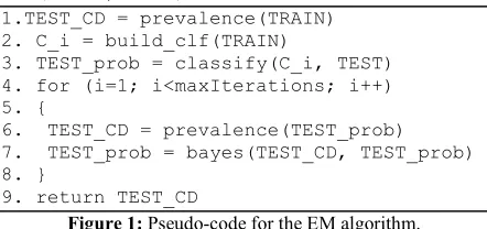
To make the Expectation Maximization (EM) meth-od clear, we specify its algorithm in Figure1 using a pseudo-code. The algorithm begins with counting start values for class probability distribution, using labels on the training set TRAIN (line 1), builds an initial classifi-er C_i from the TRAIN set (line 2) and classifies each item in the unlabeled TEST set (line3), where the classify functions return the a posteriori probabili-ties (TEST_prob) for the specified datasets. The algo-rithm then iterates in lines 4-9 until the maximum num-ber of iterations (maxIterations) is reached. In this loop, the algorithm first uses the previous a posteriori probabilities TEST_prob to estimate a new a priori probability (line 6). Then, in line 7, a posteriori proba-bilities are computed using Equation (4). Finally, once the loop terminates, the last posteriori probabilities re-turns (line 9).
EM (TRAIN, TEST)
1.TEST_CD = prevalence(TRAIN) 2. C_i = build_clf(TRAIN)
3. TEST_prob = classify(C_i, TEST) 4. for (i=1; i<maxIterations; i++) 5. {
6. TEST_CD = prevalence(TEST_prob) 7. TEST_prob = bayes(TEST_CD, TEST_prob) 8. }
9. return TEST_CD
Figure 1: Pseudo-code for the EM algorithm.
To build a classifier in the function build_clf, we use support vector machines (SVM) with linear kernel.
2.6
Iterative Class Distribution EstimationAnother interesting method is iterative cost-sensitive class distribution estimation (CDEIterate) described in the study by (Xue and Weiss, 2009).
The main idea of this method is to retrain a classifier at each iteration, where the iterations progressively im-prove the quantification accuracy of performing the «classify and count» method via the generated cost-sensitive classifiers.
For the CDE-based method, the final prevalence is induced from the TRAIN labeled set with the cost of classes COST. The COST value is computed with Equa-tion (5), utilizing the class distribuEqua-tion calculated during the previous step TEST_CD. For each iteration, we re-calculate:
= _
_ (5)
The CDEIterate algorithm is specified in Figure 2, using the pseudo-code. The algorithm begins with counting the class distribution TRAIN_CD for training labels TRAIN (line 1). Then it builds an initial classifier C_i from the TRAIN set (line 2). In a loop, this algo-rithm uses the previous classifier C_i to classify the unlabeled TEST set by estimating a posterior probabil-ity TEST_prob for each item in a test set (line 5). Then. in line 6, the a priory probability distribution is computed and the cost ratio information is updated (line 7). In line 8, a new cost-sensitive classifier C_i is gen-erated using the TRAIN set with the updated cost ratioCOST. The algorithm then iterates in lines 4-9 until the maximum number of iterations (maxIterations) is reached. Finally, once the loop terminates, the last a priory probability distribution of classes is returned TEST_CD (line 10).
CDEIterate (TRAIN, TEST, COST_start) 1.TRAIN_CD = prevalence(TRAIN)
2. C_i = build_clf(TRAIN, COST_start) 3. for (i=1; i<maxIterations; i++) 4. {
5. TEST_prob= classify(C_i, TEST) 6. TEST_CD = prevalence(TEST_prob) 7. COST = TEST_CD/TRAIN_CD
8.C_i = build_clf(TRAIN, COST) 9. }
[image:3.612.78.299.344.448.2]10. return TEST_CD
Figure 2: Pseudo-code for the CDE-Iterate algorithm.
To build a cost-sensitive classifier in the function
build_clf, we tried a few ones and chose a fast
lo-gistic regression classifier.
We did not find any open library where baseline quantification methods were implemented. We, there-fore, shared all the algorithms, which we had pro-grammed using the Python language, on the Github re-pository1. We believe that this library can help pool in-formation on quantification.
3
Experiment MethodologyThis section describes our experimental setup. It de-scribes the datasets we use, the specific experiments we run and the classifier induction algorithm we employ.
3.1
Simulations on Artificial DataWe present a simple experiment that illustrates the effi-ciency of iterative adjustment of the a priori probabili-ties.
1
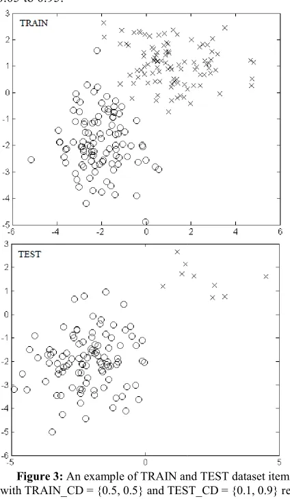
We use random sample generators from SkiKit Library to build artificial datasets of controlled size and complexity2. For each dataset we generate 10
ords with 10 features. Figure 3 exemplifies a dataset with two classes.
The initial prevalence for classes
(ptrain(c1) = ptrain(c2) = 0.5). The total set randomly splits into two subsets: 25% training set, 75% test set. training set, the class distribution remains unchanged. For the test set, we vary prevalence value
[image:4.612.81.293.204.568.2]0.05 to 0.95.
Figure 3: An example of TRAIN and TEST
with TRAIN_CD = {0.5, 0.5} and TEST_CD spectively (generated with 2 fea
For each prevalence value we generate a ferent test sets. Therefore, nineteen hundred of the following experimental design are applied.
We used a Kullback-Leibler Divergence (KLD) tween the true class prevalence and the
2 http://scikit-learn.org/stable/modules/generated/sklearn.da sification.html
erators from SkiKit-Learn Library to build artificial datasets of controlled size and dataset we generate 10,000
rec-exemplifies 2 features of
es c1 and c2 was equal otal set randomly splits into two subsets: 25% training set, 75% test set. For the training set, the class distribution remains unchanged. prevalence value (c1) from
and TEST dataset items {0.5, 0.5} and TEST_CD = {0.1, 0.9} re-spectively (generated with 2 features).
For each prevalence value we generate a hundred dif-nineteen hundred replications of the following experimental design are applied.
Leibler Divergence (KLD) be-tween the true class prevalence and the predicted class
learn.org/stable/modules/generated/sklearn.datasets.make_clas
prevalence as a quality evaluation metrics for quantif ers.
3.2
Test DatasetTo evaluate the algorithms on the real data
pated in the SemEval-2016 Task 4 called “Sentiment Analysis in Twitter”. Its dataset consists of
sages (aka observations) divided Task 4 consists of five subtasks, but w
ed in subtasks D and E: tweet quantification according to a two-point scale and five
These subtasks are evaluated
topics, and the final result is counted as an average of evaluation measure out of all the topics
2016).
The organizers provide a default split of the data into training, development and development
tasets. The algorithms evaluation is performed these subsets. The training subset is used as a TRAIN set, development and development
are used as a TEST set.
Since observation x in this dataset is a message wri ten in a natural language, we first need to transform it to the vector representation X. Based on a study by and Sebastiani, 2015), we choose the following comp nents of the feature vector:
TFIDF for word n-grams with n 4
TFIDF character n-grams where n 5.
Feature vector is extracted with a We also perform data preprocessing terns (e.g. links, emoticons, numbers) w with their substitutes. For word n
matization using WordNetLemmatizer.
It is interesting to characterize messages using SentiWordNet library. For each token
we obtain its polarity value from the SentiWordNet. First, we recognize the part of speech using
tagger from the NLTK library
cond, we get the SentiWordNet first polarity value for this token using the part of speech information.
We used polarity values to extend vector represent tion of documents in two ways
the polarity score as a sum of positive minus negative polarity values and add this feature to tor representation of a document. Second the sum of positive polarities and
3 http://scikit-learn.org/stable/modules/generated/sklearn.feature_extraction. text.TfidfVectorizer.html
a quality evaluation metrics for
quantifi-To evaluate the algorithms on the real data, we partici-2016 Task 4 called “Sentiment Its dataset consists of Twitter
mes-divided into several topics. Task 4 consists of five subtasks, but we only
participat-D and E: tweet quantification according point scale and five-point scale, respectively. independently for different final result is counted as an average of evaluation measure out of all the topics (Nakov et al.,
default split of the data into training, development and development-time testing da-tasets. The algorithms evaluation is performed using
raining subset is used as a TRAIN set, development and development-time testing subsets
in this dataset is a message writ-ten in a natural language, we first need to transform it to
. Based on a study by (Gao , we choose the following
compo-grams with n varying from 1 to
grams where n varies from 3 to
extracted with a Scikit_Learn tool3. We also perform data preprocessing .Several text
pat-links, emoticons, numbers) were replaced For word n-grams we apply lem-matization using WordNetLemmatizer.
It is interesting to characterize messages using the SentiWordNet library. For each token xi in document X
obtain its polarity value from the SentiWordNet. part of speech using a speech NLTK library (Bird et al., 2009). Se-get the SentiWordNet first polarity value for
part of speech information.
We used polarity values to extend vector representa-tion of documents in two ways: first we simply calculate
sum of positive minus a sum of negative polarity values and add this feature to the
vec-presentation of a document. Second, we calculate sum of positive polarities and the sum of negative
polarities and add these two features to the vector repre-sentation of a document.
The metrics that we use to evaluate the classifier performance are described in (Nakov et al., 2016) and are not described here.
4
Experiment ResultsWe apply six quantification methods mentioned above in Section 2: CC, PCC, ACC, PACC, EM, CDEIterate and compare them.
4.1
Synthesized DataFirst, we applied CC, PCC, ACC, PACC, EM and CDEIterate algorithms to generated data described in Section 3.1. Synthesized data allows us to perform a comparative analysis of these quantification methods with different amount of distribution drift.
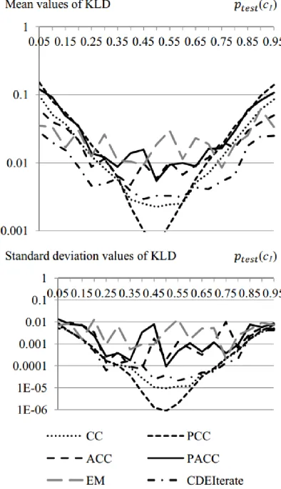
[image:5.612.316.513.217.559.2]In Figure3, which demonstrates the means and stand-ard deviation values of the evaluation measure – Kullback-Leibler Divergence (KLD), each point is ob-tained by averaging over one hundred generated da-tasets with different prevalence.
Figure 4: Mean and standard deviation values of
Kullback-Leibler Divergence for different distribution drifts in the TEST set on the linear scale.
It is obvious from Figure 4 that the CDEIterate ap-proach shows the lowest KLD mean values when a dis-tribution drift is relatively large. A standard deviation value for the CDEIterate method remains the smallest one among all possible distribution drifts.
On the contrary, the EM approach shows very unsta-ble results. Sometimes the EM algorithm converges far from the real value. Its standard deviation displays the same unstable behavior.
For more careful consideration, let us show its func-tions in the logarithmic scale in Figure 5.
Figure 5: Mean and standard deviation values of
Kullback-Leibler Divergence for different distribution drifts in the TEST set on the logarithmic scale.
When distribution changes from the starting value ptrain(c) = 0.5 by less than 0.1, the simple methods like CC and PCC show better performance (lower KLD).
4.2
Test Data [image:5.612.81.277.353.682.2]the COST_start variable to the algorithm shown in Figure 2. The first starting point is a priori probability distribution of a training set. Therefore, for the starting iteration we assume TEST_CD to equal TRAIN_CD. The second starting point is when TEST_CD is uni-formly distributed. This case is labeled as CDEIterate_U. In the previous Section 4.1, these two starting points were actually the same.
Method Quantification accuracy measure
CC 0.102469788749
ACC 0.192896311253
PCC 0.24076249451
PACC 0.23644037492
EM 0.24076249451
CDEIterate 0.101057466171
CDEIterate_U 0.0886349793929
Table1: Comparison of methods on test sample with a
two-point scale (SemEval-2016 Task4 Subtask D).
Method Quantification accuracy measure
CC 0.940764808798
ACC 0.878280429893
PCC 1.02616631747
PACC 1.04546915144
EM 1.12790745311
CDEIterate 0.538279399063
[image:6.612.90.290.184.270.2]CDEIterate_U 0.536691406139
Table 2: Comparison of methods ontest sample with a
five-point scale (SemEval-2016 Task4 Subtask E).
CDEIterate_U approach showed the best accuracy on the testing set among others with both five-point and two-point scales.
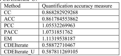
SentiWordNet is usually regarded as an important source of information about word sentiment (Baccianella et al., 2010; Esuli and Sebastiani, 2006). In our comparison, we add the sum of positive scores and the sum of negative scores of each word as two addi-tional features to the feature vector. Only the first mean-ing, according to the recognized part of speech, was used. The quantification methods remain the same. The results provided in Table 3, show that the new features increase quantification accuracy for CC, ACC, but sur-prisingly decrease it for PCC, PACC, EM, CDEIterate and CDEIterate-U.
Method Quantification accuracy measure
CC 0.868282929268
ACC 0.861784553862
PCC 1.05532269963
PACC 1.0731851762
EM 1.11319538187
CDEIterate 0.58872710467
[image:6.612.88.292.188.403.2]CDEIterate_U 0.587811269105
Table 3: Comparison of methods on test sample with a
five-point scale with additional SentiWordNet features (SemEval-2016 Task4 Subtask E).
We explain this behavior as follows: simple algo-rithms cannot adjust to the whole singularity and such additional features increase dimension and, thereby, ac-curacy. In a more complex case, the classifier extracts information from features more efficiently. Additional information about polarity scores leads to algorithm overtraining. We can guess that, as tweets contain crea-tive spelling and abbreviation common in Twitter (like “lol”, not presented in SentiWordNet), the existence of character n-grams contains more specific information than polarity scores of selected, properly written words. Therefore, we exclude SentiWordNet features from the final feature vector.
5
Conclusion and future workThe aim of this research was to perform comparative analysis of different approaches of state-of-the-art quan-tification techniques.
For tweet quantification on a five-point scale (Sub-task E) and a two-point scale (Sub(Sub-task D), the best per-formance was demonstrated by the adopted iterative method proposed by (Xue and Weiss, 2009), based on the iterative procedure with the cost-sensitive supervise learner. All the algorithms mentioned in the article, are available on the Github repository4.
In our future work, we are planning to move in two directions. First, we plan to extend the vector of features used for representation of documents. Second, we want to add more quantification methods to our open source library.
Acknowledgments
The reported study was funded by RFBR under research Project No. 16-06-00184 A.
References
Stefano Baccianella, Andrea Esuli, and Fabrizio Sebastiani. 2010. SentiWordNet 3.0: An Enhanced Lex-ical Resource for Sentiment Analysis and Opinion Min-ing. In LREC, volume 10, pages 2200–2204.
Steven Bird, Ewan Klein, and Edward Loper. 2009.
Natural language processing with Python. O’Reilly Media, Inc.
Yee Seng Chan and Hwee Tou Ng. 2006. Estimating class priors in domain adaptation for word sense disam-biguation. In Proceedings of the 21st International Con-ference on Computational Linguistics and the 44th
4
[image:6.612.91.290.589.681.2]nual meeting of the Association for Computational Lin-guistics, pages 89–96. Association for Computational Linguistics.
Andrea Esuli and Fabrizio Sebastiani. 2006.
Sentiwordnet: A publicly available lexical resource for opinion mining. In Proceedings of LREC, volume 6, pages 417–422. Citeseer.
Andrea Esuli, Fabrizio Sebastiani, and Ahmed ABBASI. 2010. Sentiment quantification. IEEE intelli-gent systems, 25(4):72–79.
George Forman. 2005. Counting positives accurately despite inaccurate classification. In Machine Learning: ECML 2005, pages 564–575. Springer. bibtex: for-man2005counting.
George Forman. 2008. Quantifying counts and costs via classification. Data Mining and Knowledge Discovery, 17(2):164–206, June.
George Forman, Evan Kirshenbaum, and Jaap Suermondt. 2006. Pragmatic text mining: minimizing human effort to quantify many issues in call logs. In
Proceedings of the 12th ACM SIGKDD international conference on Knowledge discovery and data mining, pages 852–861. ACM.
Wei Gao and Fabrizio Sebastiani. 2015. Tweet Senti-ment: From Classification to Quantification. In Pro-ceedings of the 2015 IEEE/ACM International Confer-ence on Advances in Social Networks Analysis and Min-ing 2015, pages 97–104. ACM. bibtex: gao2015tweet.
A. Guerrero-Curieses, R. Alaiz-Rodriguez, and J. Cid-Sueiro. 2009. Cost-sensitive and modular land-cover classification based on posterior probability estimates.
International Journal of Remote Sensing, 30(22):5877– 5899.
David J. Hand and others. 2006. Classifier technology and the illusion of progress. Statistical science, 21(1):1– 14.
Preslav Nakov, Alan Ritter, Sara Rosenthal, Veselin Stoyanov, and Fabrizio Sebastiani. 2016. SemEval-2016 Task 4: Sentiment Analysis in Twitter. In Proceedings of the 10th International Workshop on Semantic Eval-uation (SemEval 2016), San Diego, California, June. Association for Computational Linguistics. bibtex: SemEval:2016:task4.
Marco Saerens, Patrice Latinne, and Christine
Decaestecker. 2002. Adjusting the outputs of a classifier
to new a priori probabilities: a simple procedure. Neural computation, 14(1):21–41. bibtex:
saerens2002adjusting.
Lidia Sánchez, Víctor González, Enrique Alegre, and Rocío Alaiz. 2008. Classification and quantification based on image analysis for sperm samples with uncer-tain damaged/intact cell proportions. In Image Analysis and Recognition, pages 827–836. Springer.
Lei Tang, Huiji Gao, and Huan Liu. 2010. Network quantification despite biased labels. In Proceedings of the Eighth Workshop on Mining and Learning with Graphs, pages 147–154. ACM.