SCAN : learning speaker identity from noisy sensor data

warwick.ac.uk/lib-publications

Original citation:

Lu, Chris Xiaoxuan, Wen, Hongkai, Wang, Sen, Markham, Andrew and Trigoni, Niki (2017)

SCAN : learning speaker identity from noisy sensor data. In: 16th International Conference

on Information Processing in Sensor Networks, Pittsburgh, Pennsylvania, USA, 18-21 Apr

2017 . Published in: 16th ACM/IEEE International Conference on Information Processing in

Sensor Networks (IPSN), 2017 pp. 67-78.

Permanent WRAP URL:

http://wrap.warwick.ac.uk/87168

Copyright and reuse:

The Warwick Research Archive Portal (WRAP) makes this work by researchers of the

University of Warwick available open access under the following conditions. Copyright ©

and all moral rights to the version of the paper presented here belong to the individual

author(s) and/or other copyright owners. To the extent reasonable and practicable the

material made available in WRAP has been checked for eligibility before being made

available.

Copies of full items can be used for personal research or study, educational, or not-for profit

purposes without prior permission or charge. Provided that the authors, title and full

bibliographic details are credited, a hyperlink and/or URL is given for the original metadata

page and the content is not changed in any way.

Publisher’s statement:

"© ACM, 2017. This is the author's version of the work. It is posted here by permission of

ACM for your personal use. Not for redistribution. The definitive version was published in

16th ACM/IEEE International Conference on Information Processing in Sensor Networks

(IPSN), 2017 pp. 67-78.

http://doi.org/10.1145/3055031.3055073

A note on versions:

The version presented here may differ from the published version or, version of record, if

you wish to cite this item you are advised to consult the publisher’s version. Please see the

‘permanent WRAP URL’ above for details on accessing the published version and note that

access may require a subscription.

Chris Xiaoxuan Lu

Department of Computer Science University of Oxford

OX1 3QD, UK [email protected]

Hongkai Wen

Department of Computer Science University of Warwick

CV4 7AL, UK

[email protected]

Sen Wang

Department of Computer Science University of Oxford

OX1 3QD, UK [email protected]

Andrew Markham

Department of Computer Science University of Oxford

OX1 3QD, UK [email protected]

Niki Trigoni

Department of Computer Science University of Oxford

OX1 3QD, UK [email protected]

ABSTRACT

Sensor data acquired from multiple sensors simultaneously is fea-turing increasingly in our evermore pervasive world. Buildings can be made smarter and more efficient, spaces more responsive to users. A fundamental building block towards smart spaces is the ability to understand who is present in a certain area. A ubiqui-tous way of detecting this is to exploit the unique vocal features as people interact with one another. As an example, consider audio features sampled during a meeting, yielding a noisy set of possible voiceprints. With a number of meetings and knowledge of partici-pation (e.g. through a calendar or MAC address), can we learn to associate a specific identity with a particular voiceprint? Obviously enrolling users into a biometric database is time-consuming and not robust to vocal deviations over time. To address this problem, the standard approach is to perform a clustering step (e.g. of audio data) followed by a data association step, when identity-rich sensor data is available. In this paper we show that this approach is not ro-bust to noise in either type of sensor stream; to tackle this issue we propose a novel algorithm that jointly optimises the clustering and association process yielding up to three times higher identification precision than approaches that execute these steps sequentially. We demonstrate the performance benefits of our approach in two case studies, one with acoustic and MAC datasets that we collected from meetings in a non-residential building, and another from an online dataset from recorded radio interviews.

CCS CONCEPTS

•Computer systems organization→Embedded systems;

Re-dundancy;Robotics; •Networks→Network reliability;

KEYWORDS

Speaker identification, data-association.

Permission to make digital or hard copies of all or part of this work for personal or classroom use is granted without fee provided that copies are not made or distributed for profit or commercial advantage and that copies bear this notice and the full citation on the first page. Copyrights for components of this work owned by others than ACM must be honored. Abstracting with credit is permitted. To copy otherwise, or republish, to post on servers or to redistribute to lists, requires prior specific permission and/or a fee. Request permissions from [email protected].

IPSN 2017, Pittsburgh, PA USA

© 2017 ACM. 978-1-4503-4890-4/17/04...$15.00 DOI: http://dx.doi.org/10.1145/3055031.3055073

ACM Reference format:

Chris Xiaoxuan Lu, Hongkai Wen, Sen Wang, Andrew Markham, and Niki Trigoni. 2017. SCAN: Learning Speaker Identity From Noisy Sensor Data. InProceedings of The 16th ACM/IEEE International Conference on Information Processing in Sensor Networks, Pittsburgh, PA USA, April (IPSN 2017),12 pages.

DOI: http://dx.doi.org/10.1145/3055031.3055073

1

INTRODUCTION

The key to reactive and personalisable behavior in smart spaces of the future is knowing who is using a particular area. Buildings and appliances can then react dynamically to demand, control heating and lighting and simultaneously improve comfort and energy effi-ciency. For such a system to be widely used, it needs to be accurate, robust and ubiquitous.

At a high level of abstraction, there are two classes of obser-vations which can be made about who is where: those which are

!"#$%&$'(!" )*%+,%-.'(

/012"(!32*.'(

#" #$ #%

!"#$%&$'(!$ )*%+,%-.'(

/012"(!32*.'(

#" #&

!"#$%&$'(!% )*%+,%-.'

/012"(!32*.'(

#&

#%

#" #'

()*)+,)

!"#$%&$'(! -)*%+,%-.'

/012"(!32*.'

. . . /01201

!"#$%&$'(! -)*%+,%-.'(

/012"(!32*.'

#" #$ #&

3456)

directly linked to theuser(identity-related observations) and those

which are linked to thecontext like a particular meeting room

(context-related observations). Identity-related observations typi-cally require active participation from the user, often in the form of carrying a device or identifying token, such as a smartphone or RFID-enabled card. Although these systems are often highly accu-rate, they are inherently not robust as a strong assumption is made that the token and user are inseparable i.e. the token is a proxy for a user. As soon as the token and the user are separated, e.g. if they lose, forget or don’t charge their token, this assumption collapses, leading to an unresponsive and brittle system. On the other hand, context-related observations such as voices of the users passively sensed in a particular space, e.g. an office, cannot be linked directly to the user identities without explicit initial enrollment into a data-base. However, the enrollment process is typically time-consuming and expensive, and needs to be constantly updated over time.

In this work, we propose associating uniquely identifiable sen-sor observations (e.g. MAC address), when available, with noisy, infrastructure-based observations of acoustic data (human voice-prints). We build a speaker identification system which gradually associates context-linked audio observations with a specific iden-tity. In this way, existing token-driven systems can be bootstrapped with additional contextual sensing to improve the performance of the system as a whole, without the cost and effort of having to make users enroll into the system. We explicitly assume that sensor data will be noisy, and present a technique that simultaneously clus-ters and names observations, yielding accurate, zero-effort speaker identification. We show that this can further improved by iterating between clustering and naming to minimize the mismatch, yielding significantly improved results in the face of increasing levels of noise. In summary, our contributions are:

• We show that side-channel information about likely

par-ticipants in an event provides valuable, albeit noisy, clues about speaker identity.

• We propose SCAN, a novel algorithm which

simultane-ously handles clustering and association, and highlight the benefits of the algorithm compared to handling these problems in a sequential manner.

• We illustrate the impact of user diversity on the speaker identification performance of SCAN, and perform a sensi-tivity analysis as we vary its key parameters.

• We compare SCAN against competing approaches using

two case studies, one based on sensor data that we collected, and one based on a real world online sensor dataset and show 3-fold improvements in performance especially in noisy environments.

The rest of the paper is orgnised as follows. Sec. 2 formulated the identification problem considered in this paper, and Sec. 3 ex-plains how the baseline approach tackles this problem. In Sec. 4 we present the proposed simultaneous cluster and naming (SCAN) algorithm, and Sec. 5 provides two real-world application scenarios in which we implement our SCAN algorithm. Sec. 6 evaluates the SCAN algorithm, and compares its performance with the competing approaches. Sec. 7 surveys the related work, while Sec. 9 concludes the paper and outlines future directions.

I

C

I –Identities OI_{– Identity Observations}

C –Contexts OC_{–Context Observations}

O

_O

100% Known Unknown Noisy

Figure 2: Schematic illustration of the problem: Identity ob-servations have known links with identities but noisy links with contexts. Context observations have known links with contexts, but unknown links with identities. The problem studied in this paper is how to learn to infer identities from context observations.

2

PROBLEM FORMULATION

In this section, we explain the key terms in our system and define the core problem of sensor association.

Context: We follow the definition in [6] and use the termcontext

Cto broadly refer to a setting in which users interact with entities in an environment e.g. a physical visit or meeting in a room, a radio program or a teleconference.

Identities: We also assume that individuals have unique identity labelsI, such as their names, email or hardware addresses of mobile devices.

Sensor Observations: We refer to sensor observations as the in-formation resulting from individuals participating in contexts. We

distinguish between two types of sensor observations: a)

Iden-tity ObservationsOI, offering direct yet noisy information about which individual may have participated in a context; and b)Context ObservationsOC, generated by sensors directly monitoring the con-text, but without offering direct knowledge of individual identities. Identity observations for example could be obtained from calendar entries or from sniffed MAC addresses. Note that in practice,OIcan be noisy: e.g. people may miss scheduled meetings or their device may be detected in multiple rooms with different probabilities. On the other hand, examples of context observationsOC _{could be the}

audio signals recorded in a meeting. Such observations typically represent passive observations of users’ important vocal features. In the absence of training data, it is challenging to immediately associate context observations to individual identities.

Therefore, theidentification problemaddressed in this paper is: given the noisy identity observationsOI_{, find the correct mapping}

between the context observationsOCand identity labelsI, so that

in the future, context-linked observationsOC _{can be}

3

BASELINE APPROACH

Intuitively, the most important task to address the identification problem is to establish the mapping between anonymous context observationsOCand identity labelsI, with the help of noisy identity observationsOI. Standard approaches tackle this in two steps: a) in the Clustering Step, context observationsOC_{are firstly grouped}

into clusters, each of which represents the features of a single individual (e.g. voice samples); and then b) in the Data Association Step, the clusters are assigned with identities based on identity observationsOI_{(e.g. calendar entries).}

Clustering Step: Given a set of contextsC, clustering occurs at two levels: at the local level clusters are formed within a single context and then globally aggregated across contexts. At the local level, the intent is to partition the sensor stream into disjoint, non-overlapping clusters. The number of clusters can be estimated via heuristics or inferred from identity observations (i.e. calendar entries). These local clusters can then be grouped across different contexts into|I|global clusters, whereIis the set of true identities of individuals who have participated in any of the contexts. This is typically accomplished with constrained clustering techniques [1] which impose additional constraints, such as whether clusters must-link or cannot-must-link, on traditional clustering algorithms such as k-means [10], spectral clustering [20] or agglomerative clustering [2].

Data Association Step: LetEGk be the membership vector of thek-th global clusterG_k. EGk[j] is set to 1 only ifGk contains observations from contextCj (see Fig. 3 for an example). The set

of contexts that contribute to clusterGk can be represented as: CGk =={Cj|EGk[j]=1}. Then, for a given identity labelIm, an edge is created betweenImandGkifImis observed to appear in

any context withinCGk, according to the identity observationsO I_.

The weight of this edge is determined by the number of contexts in CGkthatImhas participated in. Then associating identities with clusters is equivalent to solving the combinatorial optimization problem on the weighted bipartite graph, e.g. using the Hungarian algorithm [12].

Limitations of Baseline Approach: The above method addresses the identification problem in two isolated steps: context observa-tions are firstly clustered and then matched to identities by min-imizing the combinatorial mismatch. Although this approach is simple and easy to implement, it is not robust to noisy observations. Firstly, errors can occur due to the noise in context observations. For example, people’s audio may vary considerably across contexts due to illness or emotional influences [32], confusing the clustering step and causing unrecoverable knock-on effects on the ensuing as-sociation step (see Fig. 4 for an example). Secondly, errors can also occur due to noisy identity observations; these affect the number of local and global clusters, and degrade the quality of data associa-tion. In the next section, we will attempt to mitigate some of these limitations by proposing a new algorithm that jointly optimises the clustering and data association steps.

4

SIMULTANEOUS CLUSTERING AND

NAMING (SCAN)

The key insight of our algorithm is that the clustering of sensor ob-servations should not be finalised independently of and in advance

of data association, but both tasks should progress in tandem. The proposed simultaneous clustering and naming algorithm works as follows. Firstly, it compiles sensor observations as an augmented linkage tree, which succinctly encodes the hierarchical clustering plans of context observations across different contexts, and more importantly all possible data association plans given a specific clus-tering plan. Then our algorithm finds the best clusclus-tering and data association plan by solving a constrained optimisation problem on the constructed linkage tree. In the following Sec. 4.1, we show how to construct the augmented linkage tree from both the context and identity observations, while in Sec. 4.2, we explain how we jointly optimise the clustering and data association processes to improve noise immunity.

4.1

Construct the Augmented Linkage

Tree

Robust Clustering:For a given context, the proposed SCAN al-gorithm uses a similar intra-context clustering process as discussed in Sec. 3, to separate the context observations of each individual locally. However, unlike the baseline approach, which only relies on the cardinality of identity observations (i.e.|OI_j|) in contextC_j to determine the number of local clusters, our algorithm considers a more robust strategy. It evaluates the number of clusters in con-textCjas follows: max{|OI_j|,kC_j }, wherekC_j is the natural number of clusters of the context observationOC_j . In practice,kC_j can be evaluated in many ways, e.g. using average silhouette or Bayesian information criterion.

The rationale here is thatOI_j can be quite noisy. Therefore, the problem of the baseline approach (only considering|OI_j|) is that it can underestimate the number of individuals in a contextCj,

and as a result generate local clusters containing mixed voiceprint of multiple individuals. For instance, an individual may attend a meeting without updating her calendar. In that case, if we still use the number of individuals inferred from calendar data to cluster audio signals of that meeting, the voices of two different people will be inevitably grouped into one cluster. To make things worse, as we move on to group together local clusters (representing an individual’s voiceprint in one context) to larger ones (representing an individual’s voiceprint across contexts), initial clustering errors will compound and lead to global clusters that are impossible to associate correctly to individuals.

On the other hand, the proposed approach could potentially overestimate the number of individuals participating in a given context. As a result, the voiceprint of a single individual may be split into two or more local clusters. We address this problem by adding dummy identity labels into our initial setI. Since we typically have enough context observations for each individual, it is safe to remove the data associated with those dummy labels from the final results.

Context Observations Local Clusters Global Clusters

4

1 2

1

1 2 2

2 1 2

1 1

E = [1, 1, 1, 1]

E = [0, 1, 1, 0]

E = [0, 1, 0, 1]

E = [1, 0, 0, 0]

I2

I3

I4

Identity Observations

Clustering Step

Data Association Step

I1

G1

G3

G4

G2

I1 I4 I1 I2 I3 I1 I2 I1 I3

O1I O

I

2 O

I

3 O

I

4 G2

G1 G3 G4

G1

G₃

G4

G₂

OC1 O

C

2 O

C

3 O

C

4

Figure 3: Illustration of the baseline approach in an example with four people and four contexts.

utterances in happy states

utterances in sad states

v

o

ic

e

fea

t

u

r

e

s

Figure 4: Deviations of voices due to the different emotion states of the speaker.

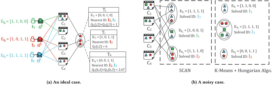
ET = [0, 0, 1, 0]

Nearest ID: I2, I3

QA(j,2)=QA(j,3) = 1

Tj

ET = [1, 0, 1, 1]

Nearest ID: I2

QA(i,2) = 6

Ti

ET = [0, 0, 1, 1] Nearest ID: I2, I3 QA(k,2)=QA(k,3) = 2.67

Tk

E = [1, 1, 1, 1] E = [1, 0, 1, 1]

E = [1, 1, 0, 0]

C2

C1

C3

C4

OI1

I1

I2 OI2

I3 OI3 I1

I2

I3

i j

k

(a) An ideal case.

E = [1, 1, 1, 1] Solved ID: I3

E = [1, 0, 0, 1] Solved ID: I1

E = [1, 1, 1, 0] Solved ID: I2

SCAN

E = [1, 1, 1, 1] Solved ID: I3

E = [1, 1, 0, 0] Solved ID: I1

E = [0, 0, 1, 1 ] Solved ID: I2

K-Means + Hungarian Algo. C2

C1

C3

C4

Ti

Tj

Tk

Ti

Tj

Tk

(b) A noisy case.

Figure 5: An example of SCAN. (a) AssigningQAto nodes in T. As the size of cluster increases, its identity becomes definite. (b) Solved global clusters by SCAN and baseline method respectively. The baseline clustering approach is conservative to deviations and messes up the identity information. SCAN is able to tolerate voice deviations and identify clusters robustly compared with the baseline method.

combination of nodes from the tree will give a specific clustering plan. For example in Fig. 6(a), selecting nodesT₁andT₄means that the local clusters in nodesT2andT3should be grouped together

(and thus belong to the same individual), whileT1is left alone as

the cluster corresponding to another individual. Each nodeTninT

is associated with alinkage scoreQ_L(n), describing the similarity between the data within the cluster it represents.

Augment Linkage Tree with Data Association Scores:Given a linkage treeT, the inter-context clustering process of the baseline approach is equivalent to finding the set of nodes inT that max-imises the total linkage score. However as discussed in the previous section, this is not reliable due to noisy sensor observations. There-fore, the proposed SCAN algorithm augments the linkage tree by introducing additional data association scores to each of its nodes Tn, which represent the fitness of assigning an identity label toTn

given identity observationsOI.

Concretely, letETn be the context membership vector of a node Tn, whereETn[j]=1 ifTncontains data collected from contextCj. Similarly, we useEIk to denote the context membership vector of an identityIk, and setEIk[j] to 1 ifIkhas participated in contextCj according to the identity observationsOI_{. Intuitively, for a nodeTn}

and an identityI_k, ifETnandEIkare similar enough, it is very likely that context observations under nodeTnare actually the voiceprint

of identityI_k, since they appear in similar series of contexts and match with each other well (as shown in Fig. 5a).

Formally, for a nodeTn, we define its data association scores with

toTn:

QA(n,k)=       

|E_T

n ⊗EIk|, ifTnis leaf

|E_Tn|[|_|E_ETn⊗EIk|

Tn⊕EIk|+

1

|E_Tn|− |E_Ik|+1], otherwise (1) where⊗and⊕are element-wise AND and OR, and| · |here is the

L1_{-norm. For a leaf node which only contains context observations}

from a single context,QA(n,k)is a binary value indicating whether individualIkhas been observed to participate in that context, given

the identity observationsOI. On the other hand for a branch node, the aboveQA(n,k)is determined by the Jaccard index and cardi-nality similarity betweenETn andEIk, i.e. it prefers to pairTnand Ikthat are associated with similar contexts. The multiplier|E_T

n| is used to favour nodes that contain data from multiple contexts, since they tend to have less ambiguity as to which identity label it should be associated with.

In this way, we augment the linkage treeT, so that each nodeTn

not only represents a candidate cluster of context observations, but also encodes all possible data association plans with corresponding scores. This means we don’t have to make the clustering decisions before assigning identities to clusters, but it is possible to jointly solve the problems of clustering and data association, which will be discussed in the next section.

4.2

Joint Optimization of Clustering and Data

Association

Given the augmented linkage treeT, the proposed SCAN algorithm aims to find the optimal clustering and data association plan simul-taneously. Essentially, we want to find the a set of|I|nodes inTand the corresponding identity assignments, which maximise: a) the similarity of the context observations clustered under each node; and b) the consistency with respect to the identity observationsOI. This can be expressed as a composite score function for each node Tn:

Q(n)=(1−ω)QL(n)+ωmax

k QA(n,k) (2)

whereQL(n)is the standard linkage score, max_kQA(n,k)is the best data association score, andωis the weight between them. As dis-cussed in Sec. 4.1, the data association scoreQA(n,k)is determined by the identity observationsOI. Therefore, here the parameterω

governs how much we trust the identity observationsOI and to

what extent we want them to impact the result of clustering. In Sec. 6.2 we will show the sensitivity of our system with respect to the parameterω, and explain how to find the optimalωin practice.

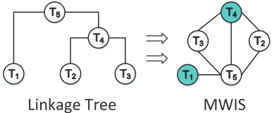
However we can’t directly optimise the sum ofQ(n)over the linkage tree, since there are certain constraints when selecting nodes from the tree, e.g. a node cannot be selected with its ancestors or descendants at the same time since they contain duplicate data. To address this, the proposed SCAN algorithm firstly converts the linkage tree to an undirected graph, where vertices are from the nodes inT, and an edge(m,n)∈Bconnects two verticesT_mandT_n if they can’t be selected at the same time (as shown in Fig. 6). Then optimisingPQ₍n₎over the_|T_|nodes is equivalent to solving the

Maximum Weighted Independent Set problem [9] on the converted

MWIS

7

7

7

7

7

7

7

7

7

7

Linkage Tree

Figure 6: Converting a linkage tree to an undirected graph where an edge connects two nodes that should not be se-lected at the same time. An example of the Maximum Weighted Independent Set (MWIS) is highlighted in green.

graph:

max

δn |T|

X

n δnQ(n)

s.t. δm+δn ≤1,∀(m,n)∈B

δm,δn ∈ {0,1}and Pδ

n =|I|

(3)

whereδn is the indicator function, andδn = 1 means then-th

node is selected. Note that here we require exactly|I|nodes to be chosen, i.e.Pδ

n=|I|. Depending on the hardness of the problem (e.g. number of nodes and the graph density), this can be solved by either exact [21] or approximate algorithms [4].

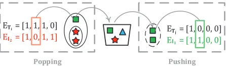
Final Cluster Refinement:Once we assign identities to global clusters, we perform a post-processing step to further refine the quality of these clusters. We revisit leaf clusters one by one, and check whether removing a leaf cluster from a global cluster could potentially increase the global cluster’s scoreQ(n). If this is the case, the leaf cluster is removed and considered as candidate to be attached elsewhere in the tree. If it cannot increase the value of any other global cluster, it is simply discarded. Otherwise, it joins the global cluster that it helps increase its fitness the most. An illustrative example is provided in Fig. 7.

It is also worth pointing out that in practice, the performance gain offered by this final cluster refinement step largely depends on the quality of identity observationsOI. If the observedOIis very trustworthy, e.g. in our experiments (Sec. 6) when erroneous iden-tity observations account for less than 10∼15% of all observations, such a refinement step is beneficial. In this case, we can safely rely on the accurate identity observations totidy upthe resulting global clusters from spurious local clusters that are inconsistent with the observedOI_{. However, if the identity observationsO}I _{are noisy,}

e.g. when>30% ofOI _{is wrong, it is better to skip this step. In}

practice, it is often difficult to determine the precise “noisiness” of the identity observations, but such information could be available as prior knowledge in different application scenarios. For example, the identity observations collected from calendar data should be more accurate than those sensed from WiFi MAC address sniffing.

4.3

SCAN vs. Online Inference

E = [1, 1, 1, 0]Ti

E = [1, 0, 1, 1]I2

E = [1, 0, 0, 0]Tj

E = [1, 1, 0, 0]I1

, ,

, ,

Popping Pushing

Figure 7: Final cluster refinement: Example of moving a lo-cal cluster from one global cluster to another in order to in-crease the fitness of both global clusters.

used for online user identification based purely on context observa-tions, without relying on identity observations. An entry in such a database maps a user’s identity to the global cluster of context observations previously generated by that user. Note that these entries are generated directly from the output of SCAN.

A classification technique, such ask-nearest neighbor algorithm, can then be used to take a sample context observation in a new pre-viously unseen context, and identify the user in the database that has the closest match. This inference step can be implemented using a variety of existing classification techniques, while the novelty of this paper lies in the proposed SCAN algorithm, which enables the building of an accurate voiceprint database even in the presence of noisy context and identity observations. The accuracy of the database has an obvious direct influence on the accuracy of the online inference step. As a consequence, SCAN enables reliable identification of users in new contexts where we possess no prior in-formation on attendance. Therefore smart spaces can learn to react to speakers even when they are not carrying explicitly identifying tokens.

5

APPLICATION SCENARIOS

Case studies:We evaluate the proposed and competing approaches in two case studies, one using sensor observations generated from physical meetings, and another from broadcast radio programs. In both cases, we assume the context observationsOCare the recorded voice clips of the participants, while the identity observationsOI

are generated from additional side channels discussed below. (1) Non-residential building meetings: The first is a number of

meetings in an office environment. The audio collection application runs on Motorola Nexus 6, which is an Android based smartphone. We organize a cohort of 16 participants who agree to share the MAC addresses of their phones and record their voices in meetings1. Five of them are selected as meeting organizers, who are responsible for organizing meetings for participants, recording audio and sharing corresponding calendar information (participant list, location, time). In this scenario, the collected calendar entries are considered to be the identity observationsOI, since they provide noisy information on the identity of participants in different meetings. There are 35 meetings recorded for voice indexing (training) and 15 meetings for online inference (testing), totalling over 30 hours of audio, recorded over a month from 6 different locations.

1_{Ethical approval for carrying out this experiment has been granted.}

The average size of a meeting is∼3 participants. Our goal in this case is to identify speakers in various meetings by their voices. To obtain the ground truth, we first segment each audio clip into segments based on speaker-change points and then manually label each segment by listening. (2) Radio programs:The second is the BBC ‘Six Minutes Eng-lish’ radio interview. There are usually 2 or 3 hosts plus 1 or 2 interviewees in one program. The text-based metadata of the interviews (e.g. transcripts) is used to generate the identity observationsOI_{. In this case, the transcripts of}

interviews are considered as the ground truth, where for each session we assume the corresponding transcript con-tains true information about its participants. Therefore in our experiments, we manually add different levels of noise to simulate noisy identity observations. 30 clips are used to learn the mapping and another 12 are used for online inference. As no interviewee takes part in more than one episode, they essentially act as spurious noisy clusters and hence we only report on the mapping between the hosts and their voices.

Our goal in both cases is to build up a voice database between voice features and speakers, and use the developed database to infer speaker identities given their voices online. Speaker identification via little human calibration is a popular but unsolved problem. The challenge here lies in that human voices across scenarios and occasions could vary significantly [16]. We briefly introduce the concept of speaker diarization below, since it is a pre-processing step for our case studies and its output serves as input to the SCAN and competing algorithms.

Speaker DiarizationAs shown in Fig. 8, speaker diarization is a process of partitioning an input audio stream into homogeneous segments according to the speaker identities [28]. The pipeline of ani-vector based speaker diarization approach used in this paper is as follows. The raw audio signal is firstly pprocessed to re-move non-informative components, such as silent gaps, background and high-frequency noise. The processed audio is then segmented into short clips based on inflection points, so that each of them is likely to only contain the utterances of a single speaker. For each clip, we extract itsi-vectors [5] as features, which are shown to be the state-of-the-art representation in various speech processing tasks [8, 25]. Then the rawi-vectors (typically∼500 dimensions) are projected to lower dimensionali-vectors (contain only the most variable 200 dimensions) using a PCA-based dimensionality reduc-tion technique [24], to account for the intra-conversareduc-tion variability of the audio data. Finally, the audio clips are grouped into local clusters based on theiri-vector features, which is essentially the intra-context clustering as discussed in Sections 3 and 4.

6

EVALUATION

UBM Training

i-vector Development CMVN

MFCC Extraction

Voicing Activity Detection Audios

Dimension Reduction Speaker Diarization

SCAN/ Baselines

Intra-context Clustering

Figure 8: Pipeline of speaker diarization. MFCC: Mel-frequency cepstral coefficients; CMVN: cepstral mean and variance normalization; GMM: Gaussian mixture model. Dimension reduction is a key step to reject noises and improve accuracy.

2 3 4 5

Number of speakers

0.8 0.9 1

F

Score

Figure 9: Evaluation of Speaker Diarization

the proposed SCAN algorithm and perform a sensitivity analysis of the algorithm as we vary the quality of the input as well as some of its key parameters. In the third part, we investigate how SCAN fares compared to state of the art competing approaches and show the benefits of using simultaneous clustering and data association to fuse context and identity observations. The last part of the evaluation focuses on the online speaker identification step, which exploits the high quality voice database generated SCAN to recognise a speaker only based on context observations (without identity observations).

6.1

Evaluation of Speaker Diarization

Speaker diarization is the preprocessing step and its performance determines the quality of local clusters, which can further affect the accuracy of SCAN and competing methods. We implement the state-of-the-arti-vector based approach [24], and in this section we evaluate its performance with / without dimensionality reduction. We consider theF₁score as a standard performance metric, which is the harmonic mean of precision and recall of speaker diarization - widely used in speaker diarization [18, 19].

F1=2· precision·recall

precision+recall (4)

Fig. 9 shows the results of speaker diarization with and with-out dimensionality reduction oni-vector features. As expected, diarization with dimensionality reduction consistently outperforms the standard approach in both cases and for various numbers of speakers. More specifically, theF₁score is improved by∼5.2% and ∼6.5% in the radio program and meeting scenarios respectively. As expected,F₁score decreases with the increase of number of speak-ers in a convspeak-ersation, but not abruptly. Therefore, for both cases, this pre-processing step can generate local clusters with reasonable

levels of noise, which serves as the input to the proposed SCAN and competing approaches.

6.2

Sensitivity Analysis of SCAN

Now we focus on the performance of the proposed SCAN algorithm and its sensitivity to parameter settings and input with different noise levels. The key performance metric here is theF1scorewhich weights recall and precision equally.

Impact of Weights Between Linkage and Association Score: The first experiment is designed to explore the impact of the level of trust that we place on the identity observations. Recall that identity observations provide a noisy prior on the attendance of participants in a context, and are derived in our use cases from sniffed MAC addresses or the radio program metadata. In SCAN, such information is jointly optimised with the clustering of audio segments as discussed in Eq. (2). The parameterωin Eq. (2) indicates the interplay between the linkage score (derived from the context

observationsOC) and data association score (derived from the

identity observationsOI_{). Intuitively, whenω is set to a small}

value, the identity observations have little impact on clustering and SCAN mostly relies on linkage score. This will of course have negative impact on the performance, since the valuable information encoded inOI _{is largely ignored. For instance, as shown in Fig. 10a,}

when we setω=0.1, SCAN only achieves very lowF1score: 0.24

on the radio program dataset and 0.18 on the meeting dataset. On the other hand, largeωtends to over trust the identity observations, which are often noisy in practice, leading to suboptimalF1score of

0.45 and 0.42 on two datasets respectively.

0.1 0.2 0.3 0.4 0.5 0.6 0.7 0.8 0.9 1

ω

0.2 0.4 0.6 0.8 1

F1

Score

Radio Program Physical Meeting

(a) Impact of choice ofω

2 3 4 5 6 7 8

Number of identities to associate

0.6 0.7 0.8 0.9 1

F1

Score

Radio Program Physical Meeting

(b) Impact of number of speakers

Location Gender First language

Affecting factors

0.6 0.7 0.8 0.9 1

F1

Score

Diverse Non-diverse

(c) Sensitivity to diversity

Figure 10: Sensitivity analysis of SCAN on physical meeting dataset.

participants per context on both datasets. An explanation for this is that when the number of distinct identities increase, the chance that two or more identities (i.e. speakers) have similar voicepoint increases. In that case, SCAN may develop incorrect linkage tree branches due to the voice similarity between users, and thus makes wrong association decisions.

Impact of Diversity of Participants:The effectiveness of SCAN in fusing context and identity observations does not depend only on the number of context participants but also on their diversity. The last experiment is designed to look at diversity through the lens of 1) recording location (relative to speaker location), 2) speaker gender and 3) first-language. Here we focus on the meeting scenario because its participants have sufficient levels of diversity.

Fig.10c shows that diversity in location of the speaker relative to the microphone can reduceF₁score by 15%. The reason is that it confuses the linkage score in the clustering process, which is partly influenced by the distance between microphone and speaker. On the other hand, gender diversity is helpful (for a given number of participants) as it makes voices from participants of different genders easier to separate. The same applies for first language of the speakers. In contexts with international students, SCAN was more accurate than in contexts with native English speakers only, for a similar reason as the one discussed in the case of gender diversity. Although diversity in gender and first language helps, SCAN remains very accurate (0.86) even in the non-diverse cases.

6.3

Comparison of SCAN with Competing

Approaches

After analysing in detail the performance of SCAN, we now proceed to compare it against a number of competing approaches. They fol-low a similar pipeline as discussed in Sec. 3. For the association step, they all use the Hungarian algorithm, but for the clustering step we consider three different clustering algorithms namely: spectral clustering,k-means and agglomerative clustering. In the following graphs, for brevity, we refer to them by the name of the clustering algorithm that they use, but remind the reader that they also include the association step.

6.3.1 Robustness to Noise.As discussed in Sec. 2, both context

and identity observations can be noisy. In the case of acoustic data, the context observations can merge clusters between different speakers or split a speaker’s voiceprint into two or more clusters. The causes of such type of noise can range from the collection environment (e.g. distance from microphone or ambient noise) to two speakers who may sound very similar. Identity noise comes

from incorrect observation of participation and can again add extra identities or remove them from the association step. These are common sources of disturbance in real-world pervasive data, and in this section we compare the performance of SCAN against baseline approaches in terms of noise immunity.

We first analyse the robustness of SCAN in two common sce-narios: a) accurate identity observations and b) noisy identity ob-servations. There are three sub-datasets in the radio program case, each of which corresponds to a particular host’s episodes. On the other hand, there are five sub-datasets in the meeting case, each of which corresponds to audio recorded by the same meeting orga-nizer. SCAN is examined on all these sub-datasets and the average F₁score is reported on both cases respectively.

Scenario 1: Accurate Identity Observations:In this setting, we validate the robustness of SCAN when faced with increasing levels of vocal deviation across contexts. To only focus on the impact of noise in context observations, we use the ground truth identity ob-servations. From the ground truth data, a centroidi-vector feature is first derived by averaging all voice samples across all contexts. The variance of all thei-vectors in terms of cosine distance [25] is denoted as the strength of vocal deviation. We split our dataset into five levels of deviation, ranging fromlevel₁with low deviation and level5with the highest deviation. Within each category,

conversa-tions are formed from those vocal samples in the same category. Note that this deviation based categorization is implemented from the dataset itself. The meetings dataset naturally suffers from higher levels of deviation due to environmental dynamics and microphone placement.

As shown in Fig. 11, the greater the deviation, the more signifi-cantly that SCAN outperforms baseline approaches. On average, SCAN has a performance of 0.85 and 0.83 on the two scenarios respectively. Even in the most extreme case (level5), SCAN is still

able to be as accurate as 0.81 and 0.70. On the other hand, the F1score of baseline approaches is below 0.6 in the radio program

Level₁ Level₂ Level₃ Level₄ Level₅

Voice Deviation Intensity

0.2 0.4 0.6 0.8 1

F1

Score

Spectral clustering K-Means Agglomerative merging SCAN w/o refinement SCAN full-version

Level₁ Level₂ Level₃ Level₄ Level₅

Voice Deviation Intensity

0.2 0.4 0.6 0.8 1

F1

Score

Spectral clustering K-Means Agglomerative merging SCAN w/o refinement SCAN full-version

Figure 11: Impact of different level of voice deviation. Left: radio program dataset; Right: physical meeting dataset.

two scenarios respectively. As shown in Table 1, we see that SCAN outperforms all baseline approaches on both radio program and physical meeting datasets. In the former scenario, SCAN outper-forms the best baseline approaches by 0.23, 0.26 and 0.23 in terms of precision, recall andF1score, while in the latter case, it improves

the performance by 0.36, 0.30 and 0.35 respectively.

Methods

/Dataset PrecisionRadio ProgramRecall F-1 PrecisionPhysical MeetingRecall F-1 Spectral

Clustering 0.68 0.64 0.66 0.52 0.56 0.53

k-means 0.69 0.66 0.67 0.50 0.54 0.52

Agglomerative

Merging 0.59 0.65 0.63 0.44 0.49 0.47

SCAN

(w/o refinement) 0.85 0.87 0.85 0.83 0.84 0.83 SCAN

(full version) 0.91 0.90 0.90 0.88 0.86 0.87

Table 1: The overall performance of competing algorithms in scenario 1, where identity observations are accurate.

Methods

/datasets PrecisionRadio Program DatasetRecall F-1 PrecisionPhysical Meeting DatasetRecall F-1 Spectral

Clustering 0.45 0.41 0.43 0.36 0.31 0.34

k-means 0.42 0.38 0.41 0.35 0.30 0.32

Agglomerative

Merging 0.43 0.49 0.45 0.40 0.39 0.40

SCAN

(w/o refinement) 0.71 0.74 0.73 0.68 0.72 0.69 SCAN

(full version) 0.69 0.72 0.71 0.69 0.71 0.71

Table 2: The overall performance of competing algorithms in scenario 2, where identity observations are noisy.

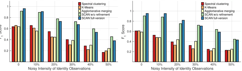
Scenario 2: Noisy Identity Observations: This scenario is much more challenging as now the uncertainties include both voiceprint deviations (i.e. we use all voices and do not split them into cate-gories) and errors in identity observations. By changing the pro-portion of correct speaker labels in conversations, we validate the

robustness of SCAN to noisy identities. There are two types of noise for identity observation, a) scheduled but absent b) present but un-scheduled. If an individual is replaced by another one this means that both types of error occur simultaneously. In this experiment, we vary the proportion of identity observation error by uniformly selecting from the two classes of error and injecting/removing an individual at random varying the proportion of identity error from 0% to 50%.

Fig. 12 shows the experimental results as identity error increases. For the radio program dataset, the three baseline methods signifi-cantly drop inF1score to below 0.25 in the case where half of the

identity observations are corrupted. It can be seen that although the precision of SCAN decreases, it degrades far more slowly than any of the the baseline approaches. TheF1score of the full version

of SCAN has decreased from 0.94 to 0.38. Interestingly, the version of SCAN without reallocation shows improved performance with high identity errors, dropping from 0.89 to 0.47. This difference is because the refinement assumes correct identity observations to move samples between clusters. Overall as shown in Table 2, SCAN performs better than all baseline algorithms, and can achieve up to 0.26, 0.25 and 0.28 improvement in precision, recall andF1score.

For the meeting dataset, the results show a similar pattern. The F1score of SCAN decreases from 0.95 and 0.86 to 0.44 and 0.47 with

and without refinement. By contrast, even with perfect identity ob-servations, the baseline methods show extremely poor performance, below 0.65 even for the best method. This is because this scenario is less controlled as audio is recorded in non-ideal environments (i.e. not in a sound-proofed recording studio) and using different phones. The resultingi-vector features are less discriminative for encapsulating biometric information. As shown in Table 2, on this dataset SCAN continues to outperform baseline approaches and the largest gain in terms of precision, recall andF1score is 0.29,

0.33 and 0.31 respectively.

0 10% 20% 30% 40% 50%

Noisy Intensity of Identity Observations

0.2 0.4 0.6 0.8 1

F1

Score

Spectral clustering K-Means

Agglomerative merging SCAN w/o refinement SCAN full-version

0 10% 20% 30% 40% 50%

Noisy Intensity of Identity Observations

0.2 0.4 0.6 0.8 1

F 1

Score

Spectral clustering K-Means

Agglomerative merging SCAN w/o refinement SCAN full-version

Figure 12: Impact of varying level of erroneous identity observations. Left: radio program dataset; Right: physical meeting dataset.

6.4

Evaluation of Online Inference

We are now in position to validate the performance of online infer-ence via the developed voice database, i.e. we now use a reserved test set of data to check our predictions of participants. By varying levels of error in identity observations, from 0% to 50% in steps of 10%, we develop six different voiceprint databases. In this experi-ment, we now focus on the overall prediction accuracy now.

The developed voiceprint database may contain certain amount of incorrect labels due to the voice deviations and noisy identity observations. Conventional PLDA classifier [3, 24] in this case is not suitable as they require reliable instance labels. We therefore use a probabilistick-Nearest Neighbor (PKNN) classifier [7], which is proved to be an effective method for the scenarios with noisy training data. It considers the uncertainties of sample labels when it trains the classifier. To assign a metric of uncertainty to a voiceprint, a voice centroid in the form ofi-vector is derived by averaging all her voice instances for each speaker in the populated database. The uncertainty of a voiceprint is then calculated by its cosine distance to its respective voice centroid [5]. Although there are other robust classifiers which can handle noisy training data, we do not discuss more in this paper because online inference is not novel but simply a implementation step to complete speaker identification.

Fig. 13 shows the end-to-end identification accuracy on two re-served test datasets. As we can see, online inference using voiceprint databases developed by SCAN (with/without) reallocation consis-tently outperforms the one developed by baseline approaches. This is as expected because the association accuracy of SCAN is much higher than baseline approaches and the resultant training data is more fine-grained. The performance difference between of SCAN with or without re-allocation is small. A potential reason is that PKNN is able to tolerate certain uncertainties of labels and narrows the accuracy gap if the quality gap of databases is within small range. This observation is also found for the performance changes with different noise intensities of identity observations. When noise intensities grows from 0 to 20%, the accuracy drops on both test set are not as dramatic as the association performance drops: 3% decline of accuracy v.s. 13% loss ofF1score for radio program case

and 5% drop of accuracy v.s. 14% decrease ofF₁score for physical meeting case. In fact, until 20% noise, online inference by SCAN

can be as accurate as around 0.8 on both datasets. Even in the worst case where 50% identity observations are incorrect, its accuracy can still be around 0.63. Considering the fact that we develop the whole pipeline of identification (diarization, voice indexing and online inference) by weak label information (names only), the end-to-end results are extremely competitive and useful for many scenarios of populating a voiceprint database from noisy identity observations.

7

RELATED WORK

Although a great deal of work has gone into fusing sensor oberva-tions, there is less research in the area of automatically associating observations across sensor sets. In terms of data association in cyber-physical systems, a number of techniques have tackled prob-lems where there exists a correlated, temporally linked pattern between a pair of sensors e.g. between a camera and wearable sen-sors. For instance, Jung et at. [13] uses multiple trajectory tracking (MTT) to associate motion traces to people detected in the field of view (FOV) from cameras. As the accelerometer readings are accessed from id-linked wearable devices, associating motion traces to detected people uniquely identifies people in the FOV. A similar approaches is also presented in [26], where the MTT is replaced by the bipartite graph matching. In EV-Loc [27] the Hungarian algo-rithm is then used to find the best match mapping between camera measurements and WiFi measurements. By using the combination of various sensing modalities and prediction models, identification accuracy can be significantly improved [22]. Unlike our work, these approaches rely on state-based models, where both sensors are ob-serving temporally evolving systems. In our approach, detecting a MAC address does not imply that someone will be speaking at that exact instant.

0 10% 20% 30% 40% 50% Noisy Intensity of Identity Observations

0.2 0.4 0.6 0.8 1

Accuracy

Spectral clustering K-Means

Agglomerative merging SCAN w/o refinement SCAN full-version

0 10% 20% 30% 40% 50%

Noisy Intensity of Identity Observations 0.2

0.4 0.6 0.8 1

Accuracy

Spectral clustering K-Means

Agglomerative merging SCAN w/o refinement SCAN full-version

Figure 13: Online inference results. Left: radio program dataset; Right: physical meeting dataset.

labels. SpeakerSense [15] and Darwin [19] pioneer this in the field of mobile sensing. SpeakerSense collects training voices from daily contexts, e.g., phone call and one-to-one conversations. It signifi-cantly reduces the calibration efforts and exploits the pervasiveness of conversations. In parallel, Darwin adopts a hybrid speaker clas-sification, in which collaborations among phones are exploited for speaker model sharing and speaker inference. To avoid a large amount of data transfer in the sharing process, SocialWeaver [18] only involves collaborative verification in model learning phase through collaboration and uses the trained speaker models for on-line inference. A similar application is SocioPhone [14], where speaker are grouped based on a pure volume-topography-based approach to detect speakers. DopEnc [36] is recently proposed that leverages Doppler effects to first classify approaching trajectories of people and identify people encounters via voices.

Finally, SCAN aims to discover knowledge (i.e. speaker identity in this paper) from noisy sensor data, which shares the similar idea with the truth discovery in social sensing [11, 29, 30] and accuracy estimation [33, 34] techniques. Those approaches typically assume that sensor data is homogeneous but comes from multiple sources, and consider the Expectation-Maximization (EM) framework to jointly estimate the reliability/accuracy of the sources and sensor measurements in the same time. However, SCAN focuses on using heterogeneous sensor data (i.e. voiceprints and identity observa-tions) from different sensing modalities to learn their associations. A promising direction is to incorporate the truth discovery/accuracy estimation step on top of SCAN, and use the learned trustworthi-ness/accuracy to adjust the behaviour of SCAN accordingly.

8

DISCUSSION

Usability: Although the problem of speaker identification has been well studied for many years, the challenge of labelling voiceprints using observations of identity from side channels has not been con-sidered. SCAN is able to build a voice database automatically with identity data derived from pervasive sensors, whether physical (e.g. MAC) or semantic (e.g. calendar information). Those identity observations act as a catalyst for the noisy voice data, and could significantly improve the performance of speaker identification without requiring user enrolment. This could open up many new applications and services, e.g. personalisation in smart homes and targeted advertising.

Privacy: In practice, SCAN requires voice data (context obser-vations) and identity observations sensed from the users (or their

devices) to operate, which may have certain impact on user pri-vacy. For example, a user may be able to be identified without explicit consent in a new environment, if the owner has the access to the voice data of this user. Although we do not explicitly study the threat model in this paper, we note potential privacy concerns worth exploring in future work.

Limitations: SCAN also has some limitations. Firstly, it relies heavily on the diversity of identities across different sessions to work well. The intuition is that SCAN is able to identify speakers more accurately if they participate in different sequences of ses-sions, i.e. the participation patterns of speakers are diverse. On the other hand, if most of the speakers have participated in the same sessions, the performance of SCAN will degrade. In that case the identity observations are not informative and SCAN can only use speaker diarization to identify different speakers. Secondly, al-though we have shown in Sec. 6.2 how to empirically set the weight ωbetween the context observations and identity observations for our datasets, it is not clear how to generalize this to different ap-plication scenarios. This may need to take other factors such as the number of speakers, and characteristics of the sensing modali-ties into account, which is beyond the scope of the current SCAN. Finally, the current version of SCAN does not have a principled mechanism to handle the ‘new comer’ scenarios, i.e. when a new speaker with no identity information is joining the session. In this case, SCAN tends to mis-associate her voices to that of a known speaker. If this only happens occasionally, we can manually remove those outliers after the voice database has been constructed. In the future we will extend SCAN to consider how to grow/modify the existing database as users join and leave.

9

CONCLUSION

ACKNOWLEDGMENTS

The authors would like to acknowledge the support of the EPSRC through grants EP/J012017/1, EP/M017583/1, EP/M019918/1 and Oxford-Google DeepMind Graduate Scholarship. We thank Yu Tang, the anonymous reviewers and our shepherd Dr. Dong Wang for their helpful comments.

REFERENCES

[1] Sugato Basu, Arindam Banerjee, and Raymond J Mooney. 2004. Active Semi-Supervision for Pairwise Constrained Clustering.. InSIAM SDM.

[2] Doug Beeferman and Adam Berger. 2000. Agglomerative clustering of a search engine query log. InProceedings of the sixth ACM SIGKDD international conference on Knowledge discovery and data mining.

[3] Bengt J Borgstr¨om and Alan McCree. 2013. Discriminatively trained bayesian speaker comparison of i-vectors. InICASSP.

[4] Stanislav Busygin. 2006. A new trust region technique for the maximum weight clique problem.Discrete Applied Mathematics(2006).

[5] Najim Dehak and et al. 2011. Front-end factor analysis for speaker verification.

IEEE Transactions on Audio, Speech, and Language Processing(2011). [6] Anind K Dey. 2001. Understanding and using context.Personal and ubiquitous

computing(2001).

[7] Benoˆıt Fr´enay and Michel Verleysen. 2014. Classification in the presence of label noise: a survey. IEEE Transactions on Neural Networks and Learning Systems

(2014).

[8] Daniel Garcia-Romero, Xinhui Zhou, and Carol Y Espy-Wilson. 2012. Multi-condition training of Gaussian PLDA models in i-vector space for noise and reverberation robust speaker recognition. InICASSP.

[9] Fanica Gavril. 1972. Algorithms for minimum coloring, maximum clique, min-imum covering by cliques, and maxmin-imum independent set of a chordal graph.

SIAM J. Comput.(1972).

[10] John A Hartigan and Manchek A Wong. 1979. A k-means clustering algorithm.

Journal of the Royal Statistical Society. Series C (Applied Statistics)(1979).

[11] Chao Huang and Dong Wang. 2016. Topic-aware social sensing with arbitrary source dependency graphs. InIEEE IPSN.

[12] Roy Jonker and Ton Volgenant. 1986. Improving the Hungarian assignment algorithm.Operations Research Letters(1986).

[13] Deokwoo Jung, Thiago Teixeira, and Andreas Savvides. 2010. Towards coopera-tive localization of wearable sensors using accelerometers and cameras. InIEEE INFOCOM.

[14] Youngki Lee, Chulhong Min, Chanyou Hwang, Jaeung Lee, Inseok Hwang, Younghyun Ju, Chungkuk Yoo, Miri Moon, Uichin Lee, and Junehwa Song. 2013. Sociophone: Everyday face-to-face interaction monitoring platform using multi-phone sensor fusion. InACM MobiSys.

[15] Hong Lu, AJ Bernheim Brush, Bodhi Priyantha, Amy K Karlson, and Jie Liu. 2011. SpeakerSense: energy efficient unobtrusive speaker identification on mobile phones. InInternational Conference on Pervasive Computing.

[16] Hong Lu, Denise Frauendorfer, Mashfiqui Rabbi, Marianne Schmid Mast, Gokul T Chittaranjan, Andrew T Campbell, Daniel Gatica-Perez, and Tanzeem Choudhury. 2012. Stresssense: Detecting stress in unconstrained acoustic environments using smartphones. InACM UbiComp.

[17] Hong Lu, Wei Pan, Nicholas D Lane, Tanzeem Choudhury, and Andrew T Camp-bell. 2009. SoundSense: scalable sound sensing for people-centric applications on mobile phones. InACM MobiSys.

[18] Chengwen Luo and Mun Choon Chan. 2013. SocialWeaver: collaborative infer-ence of human conversation networks using smartphones. InACM SenSys.

[19] Emiliano Miluzzo, Cory T Cornelius, Ashwin Ramaswamy, Tanzeem Choudhury, Zhigang Liu, and Andrew T Campbell. 2010. Darwin phones: the evolution of sensing and inference on mobile phones. InACM MobiSys.

[20] Andrew Y Ng, Michael I Jordan, Yair Weiss, and others. 2001. On spectral clustering: Analysis and an algorithm. InNIPS.

[21] Patric RJ ¨Osterg˚ard. 2001. A new algorithm for the maximum-weight clique problem.Nordic Journal of Computing(2001).

[22] Savvas Papaioannou, Hongkai Wen, Zhuoling Xiao, Andrew Markham, and Niki Trigoni. 2015. Accurate Positioning via Cross-Modality Training. InACM SenSys.

[23] Douglas A Reynolds and Richard C Rose. 1995. Robust text-independent speaker identification using Gaussian mixture speaker models. IEEE transactions on speech and audio processing(1995).

[24] Stephen Shum, Najim Dehak, Ekapol Chuangsuwanich, Douglas A Reynolds, and James R Glass. 2011. Exploiting Intra-Conversation Variability for Speaker Diarization.. InINTERSPEECH.

[25] Stephen H Shum, Najim Dehak, R´eda Dehak, and James R Glass. 2013. Unsu-pervised methods for speaker diarization: An integrated and iterative approach.

IEEE Transactions on Audio, Speech, and Language Processing(2013). [26] Thiago Teixeira, Deokwoo Jung, and Andreas Savvides. 2010. Tasking networked

cctv cameras and mobile phones to identify and localize multiple people. InACM UbiComp.

[27] Jin Teng, Boying Zhang, Junda Zhu, Xinfeng Li, Dong Xuan, and Yuan F Zheng. 2014. Ev-loc: integrating electronic and visual signals for accurate localization.

IEEE/ACM Transactions on Networking(2014).

[28] Sue E Tranter and Douglas A Reynolds. 2006. An overview of automatic speaker diarization systems.IEEE Transactions on Audio, Speech, and Language Processing

(2006).

[29] Dong Wang, Tarek Abdelzaher, Lance Kaplan, Raghu Ganti, Shaohan Hu, and Hengchang Liu. 2013. Exploitation of physical constraints for reliable social sensing. InIEEE RTSS.

[30] Dong Wang, Lance Kaplan, Hieu Le, and Tarek Abdelzaher. 2012. On truth discovery in social sensing: A maximum likelihood estimation approach. InIEEE IPSN.

[31] He Wang, Dimitrios Lymberopoulos, and Jie Liu. 2014. Local business ambience characterization through mobile audio sensing. InACM WWW.

[32] Kunxia Wang, Ning An, Bing Nan Li, Yanyong Zhang, and Lian Li. 2015. Speech emotion recognition using Fourier parameters.IEEE Transactions on Affective Computing(2015).

[33] Hongkai Wen, Zhuoling Xiao, Andrew Markham, and Niki Trigoni. 2015. Ac-curacy estimation for sensor systems.IEEE Transactions on Mobile Computing

(2015).

[34] Hongkai Wen, Zhuoling Xiao, Niki Trigoni, and Phil Blunsom. 2013. On assessing the accuracy of positioning systems in indoor environments. InEWSN.

[35] Chenren Xu, Sugang Li, Gang Liu, Yanyong Zhang, Emiliano Miluzzo, Yih-Farn Chen, Jun Li, and Bernhard Firner. 2013. Crowd++: unsupervised speaker count with smartphones. InACM UbiComp.