warwick.ac.uk/lib-publications
Original citation:
Colcombet, Thomas , Jurdzinski, Marcin, Lazic, Ranko and Schmitz, Sylvain (2017) Perfect half
space games. In: 32nd Annual ACM/IEEE Symposium on Logic in Computer Science (LICS),
Reykjavik, Iceland, 20-23 Jun 2017. Published in: Proceedings of the 32nd Annual ACM/IEEE
Symposium on Logic in Computer Science (LICS).
Permanent WRAP URL:
http://wrap.warwick.ac.uk/87820
Copyright and reuse:
The Warwick Research Archive Portal (WRAP) makes this work by researchers of the
University of Warwick available open access under the following conditions. Copyright ©
and all moral rights to the version of the paper presented here belong to the individual
author(s) and/or other copyright owners. To the extent reasonable and practicable the
material made available in WRAP has been checked for eligibility before being made
available.
Copies of full items can be used for personal research or study, educational, or not-for profit
purposes without prior permission or charge. Provided that the authors, title and full
bibliographic details are credited, a hyperlink and/or URL is given for the original metadata
page and the content is not changed in any way.
Publisher’s statement:
“© 2017 IEEE. Personal use of this material is permitted. Permission from IEEE must be
obtained for all other uses, in any current or future media, including reprinting
/republishing this material for advertising or promotional purposes, creating new collective
works, for resale or redistribution to servers or lists, or reuse of any copyrighted component
of this work in other works.”
A note on versions:
The version presented here may differ from the published version or, version of record, if
you wish to cite this item you are advised to consult the publisher’s version. Please see the
‘permanent WRAP URL’ above for details on accessing the published version and note that
access may require a subscription.
Perfect Half Space Games
Thomas Colcombet
IRIF
CNRS & Universit´e Paris-Diderot
Marcin Jurdzi´nski
Ranko Lazi´c
DIMAP & Dpt. of Computer Science University of Warwick
Sylvain Schmitz
LSV
ENS Paris-Saclay & CNRS & INRIA Universit´e Paris-Saclay
Abstract—We introduce perfect half space games, in which the goal of Player 2 is to make the sums of encountered multi-dimensional weights diverge in a direction which is consistent with a chosen sequence of perfect half spaces (chosen dynamically by Player 2). We establish that the bounding games of Jurdzi ´nski et al. (ICALP 2015) can be reduced to perfect half space games, which in turn can be translated to the lexicographic energy games of Colcombet and Niwi ´nski, and are positionally determined in a strong sense (Player 2 can play without knowing the current perfect half space). We finally show how perfect half space games and bounding games can be employed to solve multi-dimensional energy parity games in pseudo-polynomial time when both the numbers of energy dimensions and of priorities are fixed, regardless of whether the initial credit is given as part of the input or existentially quantified. This also yields an optimal
2-EXPTIME complexity with given initial credit, where the best known upper bound was non-elementary.
I. INTRODUCTION
A d-dimensional energy game [5, 14] sees two players compete in a finite game graph, whose edges are decorated with vectors of weights inZd. Thedweights represent various discrete resources that can be consumed or replenished by the actions of the game. The objective of Player 1, given an initial credit in Nd, is to play indefinitely without depleting
any of the resources—more precisely to keep the current sum of encountered weights plus initial credit non-negative in every dimension—while Player 2 attempts to foil this. The primary motivation for these games is controller synthesis for resource-sensitive reactive systems, where they are also closely related to multi-dimensional mean-payoff games—and actually equivalent if finite-memory strategies are sought for the latter [14, Lemma 6]. But they appear in diverse settings: for example, in process algebra, they are equivalent to the simulation problem between a finite state system and a Petri net or a basic parallel process [10, Propositions 6.2 and 6.4]; in artificial intelligence, they allow to solve the model-checking problem for the resource-bounded logic RB±ATL [3, 2].
The algorithmic issues surrounding multi-dimensional energy games have come under considerable scrutiny. Deciding whether there exists an initial credit that would allow Player 1 to win iscoNP-complete [14, Theorem 3], while the complexity when the initial credit is given as part of the input becomes 2-EXPTIME-complete [10, 12]. Finally, both decision problems are in pseudo-polynomial time when dis fixed [12].
Open Questions: However, these recent advances do not settle the case of multi-dimensional energy parity games [7],
where Player 1 must ensure that, in addition to the quantita-tive energy objecquantita-tive (specifying resource consumption and replenishment), she also complies with a qualitativeω-regular objective in the form of a parity condition (specifying functional requirements). These games with arbitrary initial credit are still coNP-complete as a consequence of [7, Lemma 4]. With given initial credit, they were first proven decidable by Abdulla, Mayr, Sangnier, and Sproston [1], and used to decide both the model-checking problem for a suitable fragment of the
µ-calculus against Petri net executions and theweaksimulation problem between a finite state system and a Petri net; they also allow to decide the model-checking problem for the resource logic RB±ATL∗ [2]. As shown by Janˇcar [11],d-dimensional energy games using2ppriorities can be reduced to ‘extended’ multi-dimensional energy games of dimensiond0=defd+p, with complexity upper bounds shown earlier by Br´azdil, Janˇcar, and Kuˇcera [5] to be in (d0−1)-EXPTIME when d0 ≥2 is fixed, and in TOWER when d0 is part of the input, leaving a substantial complexity gap with the 2-EXPTIME-hardness shown in [10].
Contributions: We introduce in Section IIperfect half space games, both
• as intermediate objects in a chain of reductions from multi-dimensional energy parity games to mean-payoff games (see Figure 1), allowing us to derive new tight complexity upper bounds based on recent advances by Comin and Rizzi [9] on the complexity of mean-payoff games, and
• as a means to gain a deeper understanding of how winning
strategies in energy games are structured.
More precisely, in perfect half-space games, positions are pairs: a vertex from a d-dimensional game graph as above, together with a d-dimensionalperfect half space. The latter is a maximal salient blunt cone inQd: a union of open half spaces of dimensionsd,d−1, . . . , 1, where each is contained in the boundary of the previous one. In these games, Player 1 may not change the current perfect half space, but Player 2 may change it arbitrarily at any move. However, the goal of Player 2 is to make the sums of encountered weights diverge in a direction which is consistent with the chosen perfect half spaces; thus the greater the dimension of the component open half spaces that Player 2 varies infinitely often, the harder it is for him to win. For example, with d = 2, if Player 2 eventually settles on the perfect half space that consists of the half planex < 0 and the half line x= 0 ∧ y <0, then he wins provided the sequence of total weights is such that either
theirx-coordinates diverge to−∞, or their x-coordinates do not diverge to +∞and theiry-coordinates diverge to −∞; if however Player 2 switches between the two half lines ofx= 0
infinitely often, then he can only win in the former manner. Firstly, we show that perfect half space games can be easily translated to thelexicographic energy gamesof Colcombet and Niwi´nski [8]. The translation amounts to normalising the edge weights with respect to the current perfect half spaces, and inserting anotherddimensions in which we encode appropriate penalties for Player 2 that are imposed whenever he changes the perfect half space (cf. Section III-B). We deduce that perfect half space games are positionally determined, and moreover that Player 2 has winning strategies that are oblivious to the current perfect half space. Along the way, we provide in Section III-A a proof of the positional determinacy of lexicographic energy games, along with pseudo-polynomial complexity upper bounds for their decision problem whendis fixed, based on the recent results of Comin and Rizzi [9] for mean-payoff games.
Secondly, we establish that perfect half space games capture bounding games (cf. Section IV). The latter were central to obtaining the tight complexity upper bounds for multi-dimensional energy games [12]. They are played purely on the d-dimensional game graphs and have a simple winning condition: the goal of Player 1 is to keep the total absolute value of weights bounded (i.e., contained in some d-dimensional hypercube). One reading of this reduction is that whenever Player 2 has a winning strategy in a bounding game, he has one that ‘announces’ at every move some perfect half space and succeeds in forcing the total weights to be unbounded in a direction consistent with the infinite sequence of his announce-ments. The proof is difficult, and relies on a construction from the previous paper [12] of a winning strategy for Player 1 in the bounding game given her winning strategy in a first-cycle game featuring perfect half spaces. Composing this with our complexity bounds for lexicographic energy games gives us a new approach to solving bounding games, improving the time complexity from the previously best(|V| · kEk)O(d4)[12,
Corollary 3.2] to(|V|·kEk)O(d3), whereV is the set of vertices andkEk the maximal absolute value over the weights in the input multi-dimensional game graph (cf. Corollary IV.6).
Thirdly, building on Janˇcar’s reduction, we show how multi-dimensional energy parity games can be solved by means of bounding games (cf. Section V). For the given initial credit problem, we obtain 2-EXPTIME-completeness, closing the aforementioned complexity gap. When the dimension d
and the number of priorities 2pare fixed, we obtain that, for both arbitrary and given initial credits, the winner is decidable in pseudo-polynomial time. With arbitrary initial credit, our new bound(|V| · kEk)O((d+p)3log(d+p))improves whenp= 0
over the previously best (|V| · kEk)O(d4) [12, Theorem 3.3].
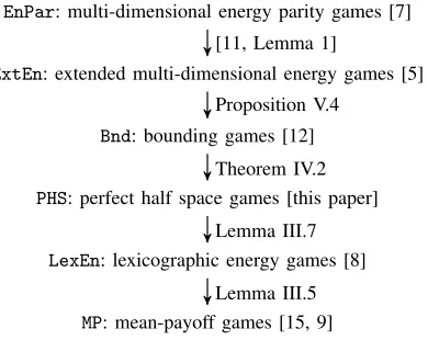
Structure of the Paper: The chain of reductions we use in this paper is depicted in Figure 1, and we shall essentially work our way up through it. In Section II we introduce multi-dimensional game graphs and perfect half space games. In Section III we show how to employ lexicographic energy games for solving perfect half space games. We apply these
EnPar: multi-dimensional energy parity games [7]
ExtEn: extended multi-dimensional energy games [5]
Bnd: bounding games [12]
PHS: perfect half space games [this paper]
LexEn: lexicographic energy games [8]
MP: mean-payoff games [15, 9]
[11, Lemma 1]
Proposition V.4
Theorem IV.2
Lemma III.7
[image:3.612.343.538.52.207.2]Lemma III.5
Fig. 1. The reductions between the various games in this paper.
results to bounding games in Section IV and multi-dimensional energy parity games in Section V, before concluding.
II. PERFECTHALFSPACEGAMES
A. Multi-Weighted Game Graphs
We considermulti-dimensional game graphswhose edges are labelled bymulti-weights, which are vectors of integers. They are tuples of the form(V, E, d), wheredis the dimension inN>0,V
def
=V1]V2is a finite set of vertices partitioned into
Player1 vertices and Player2 vertices, andE is a finite set of edges included inV ×Zd×V, such that every vertex has at
least one outgoing edge. We may write just ‘weight’ instead of ‘multi-weight’ when there is no risk of confusion, and also
v−w→v0 to denote an edge(v,w, v0). Given a path P in the game, we denote byw(P)the sum of the weights encountered. For a vectorwinZd, we letkwk= maxdef 1≤i≤d|w(i)|denote its infinity norm; we define the normkEk def
= max
v−w→v0∈Ekwk
as the maximum of the norms of edge weights. We assume all our integers to be encoded in binary, hence kEk might be exponential in the size of the multi-weighted game graph.
Without loss of generality, we assume that the players strictly alternate (v −w→ v0 in E implies v in Vi and v0 in V3−i for someiin{1,2}), the weight of every edge is determined by
its vertices (v−w→v0 andv w
0
−−→v0 in E impliesw=w0), and not all weights are zero (kEk>0).
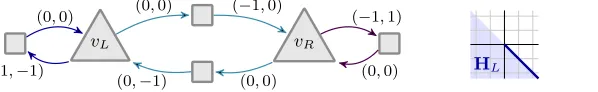
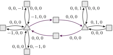
ExampleII.1. Figure 2 shows on its left-hand-side an example of a 2-dimensional weighted game graph. Throughout this paper, Player1 vertices are depicted as triangles and Player2
vertices as squares.
B. Perfect Half Spaces
vL vR (0,0) (−1,0)
(0,0) (0,−1)
(1,−1)
(0,0) (−1,1)
[image:4.612.139.438.52.98.2](0,0) HL HR
Fig. 2. A 2-dimensional game graph(V, E,2)and two perfect half spaces.
Let |H|=defk. When|H|=d, the representation is a (full) perfect half space; when |H|= 0, it is the empty set since there is only one 0-dimensional vector and the ordering≺is strict.
We define the norm kHk as the maximum of kh1k, . . . ,khkk.
Example II.2. The two perfect half spaces of interest on the right-hand side of Figure 2 are{(x, y) : x+y <0} ∪ {(x, y) :
x+y= 0∧x >0} denoted by HL def
= ((1,1),(−1,1)), and
{(x, y) : x+y < 0} ∪ {(x, y) : x+y = 0∧x < 0}
denoted by HR def
= ((1,1),(1,−1)). They have the half-plane
{(x, y) : x+y <0}with normal vector(1,1)in common, but differ on which half-line of its boundary {(x, y) : x+y= 0}
they contain.
We shall reason sometimes directly on the representations of partially perfect half spaces through theprefix ordering. We write H≤prefH0 whenH is a prefix ofH0, and lcp
iHi for the longest common prefix of a finite or infinite set of partially perfect half spaces H1,H2, . . .. Observe that, if a·H0 ≺0
andH≤prefH0, thena·H0.
C. Perfect Half Space Games
We write (V ,b E, db )for the weighted game graph obtained
from(V, E, d)by pairing vertices inV with perfect half spaces of appropriately bounded norms, which may be changed only by Player 2:
• for both i∈ {1,2},Vbi def
=Vi× Hwhere His the set of all perfect half spaces of norm at most |V| · kEk;
• Eb is the set of all(v,H) w
−→(v0,H0)such thatv−w→v0
is in E and ifv∈V1 thenH=H0.
Let PHS(V ,b E, db ) denote the perfect half space game in
which the goal of Player2 is for the total weight to diverge in a direction consistent with the chosen perfect half spaces:
Definition II.3 (Winning Condition for Perfect Half-Space Games). An infinite play (v0,H0)
w1
−−→ (v1,H1)
w2
−−→ (v2,H2)· · · iswinning for Player2if there exists a partially
perfect half space(g1, . . . ,gk)withk >0that is a prefix ofHi for all sufficiently large i, s.t.lim supnPn
j=1wj·gk =−∞ and, for all 1≤` < k,lim infnP
n
j=1wj·g`<+∞. Observe that whether Player 2 wins from(v,H)does not depend onH, hence we say that Player2wins fromv if there existsH∈ Hsuch that he wins from(v,H)—equivalently, he wins from(v,H)for allH∈ H—, and similarly for Player 1.
Given a finite path
P = (def v0,H0)
w1
−−→(v1,H1)· · ·(vn−1,Hn−1)
wn
−−→(vn,Hn)
in a perfect half space game, we denote by lcp(P) =def lcp0≤i≤nHithe longest partially perfect half space that agrees with all the perfect half spaces seen along the path. We also inherit the notation w(P)=def Pn
i=1wi that accounts for the sum of the weights inP. We say thatP is winning for Player1
ifw(P)·lcp(P)0. Similarly,P is winning for Player 2 if
w(P)·lcp(P)≺0. Note that whenP is in fact a cycle, then its infinite iteration is winning for a player if and only if the cycle is winning for them according to this definition.
ExampleII.4. Player2wins the perfect half space game on the graph of Example II.1 from any vertex by choosing the perfect half spaceHL from Example II.2 when going tovL andHR when going tovR. Indeed, either Player1 eventually only uses the left (blue) cycle, in which case(g1,g2)
def
=HL itself can be used as witness in Definition II.3, or she eventually only uses the right (violet) cycle, in which case(g1,g2)
def
=HR fits, or she alternates infinitely often between vR and vL (using the cyan cycle), in which case the partially perfect half space
(g1)
def
= ((1,1))is a witness of his victory.
III. SOLVINGPERFECTHALFSPACEGAMES
As an intermediate step towards the proof of our determinacy and complexity results for perfect half space games (Theo-rem III.8), we employ another winning condition introduced in [8]: that of lexicographic energy games. We start by presenting a proof of their positional determinacy, and an upper bound for their decision problem using the state-of-the-art results of Comin and Rizzi [9] for mean-payoff games. We then proceed to show how perfect half space games can be reduced to lexicographic energy ones in Section III-B.
A. Solving Lexicographic Energy Games
1) Lexicographic Energy Games [8] are played on multi-weighted game graphs (V, E, d), as described in Section II. An infinite playv0
w1
−−→v1
w2
−−→ · · · iswinning for Player 2 if there exists1≤k≤ds.t.lim supnPn
j=1wj(k) =−∞and,
for all1≤` < k,lim infnPnj=1wj(`)<+∞.1
Put differently, lexicographic energy games are akin to perfect half space games, except that the same full perfect half space(−e1, . . . ,−ed)is associated to every vertex of the game graph, whereei for1≤i≤d denotes the unit vector with1 in coordinateiand0 everywhere else.
1Lexicographic energy games bear a superficial resemblance to two different
ExampleIII.1. Let us consider the multi-weighted game graph of Example II.1. Player1 wins the lexicographic energy game from any initial vertex, by moving to vL and looping on the left (blue) loop.
2) Strategies: A strategy for a player is positionalif, from each of her vertices, the player using it always chooses the same outgoing edge, no matter where the play started or how it evolved so far. We say that a game ispositionally determinedif the two players have positional strategiesσandτ, respectively, such that for every vertex v ∈ V, either σ is winning for Player 1 fromv, orτ is winning for Player2 fromv.
3) Reduction to Mean-Payoff Games: Amean-payoff game is played on a weighted game graph, i.e. a 1-dimensional weighted game graph(V, E,1), and is denotedMP(V, E). From an infinite playv0
u1
−→v1
u2
−→v2· · ·, Player1(‘Max’) gains a
payofflim infn→∞(u1+· · ·+un)/n, whereas Player2(‘Min’) loses a payoff lim supn→∞(u1+· · ·+un)/n. A strategy for Max is optimalfor her if by following it she is guaranteed to gain at least as much as when using any other strategy, and optimal strategies for Min are defined symmetrically. By the positional determinacy of mean-payoff games [15], there exist positional optimal strategies for both players, yielding the same payoff for both from each initial vertex, called the valueof the vertex.
A strategy for Max is winningfrom some initial vertex if by following it she is guaranteed to gain at least≥0, and a strategy for Max is winning if by following it he is guaranteed to lose at least <0. Note that not every winning strategy for Min needs to be optimal, but that if she wins then any optimal strategy is winning: Min wins the game if and only if the value of the initial vertex is ≥0, and Max wins otherwise.
For a multi-weighted game graph (V, E, d), and for everyi,
1 ≤i ≤ d, let the set E(i) consist of the edges v −−−→w(i) v0
wherev−w→v0∈E.
Theorem III.2. (i) Lexicographic energy games are posi-tionally determined.
(ii) There is an algorithm for solving lexicographic energy games whose running time is in
O|V|d+1· |E| ·Qd
i=1kE(i)k
.
We start by describing a translation from lexicographic energy games to mean-payoff games, similar to the classical translation from parity games [13]: the idea is to write the d-dimensional weights into a single weight by shifting the most significant components by appropriate amounts. We define accordingly the sets of weighted edges E(i) for
i=d, d−1, . . . ,1as follows:
• E(d)=defE(d);
• for all i=d−1, d−2, . . . ,1, and for all v−w→v0 ∈E, if v −−−→ri+1 v0 ∈ E(i+1) then v ri
−→ v0 ∈ E(i), where
ri def
=w(i)· |V| · kE(i+1)k+ 1
+ri+1.
We will argue directly that positional optimal strategies for the two players in the mean-payoff game MP(V, E(1)) witness
positional determinacy of the lexicographic energy game
LexEn(V, E, d).
vL vR
0 −7
0
−1 6
0 −6
[image:5.612.338.537.51.95.2]0
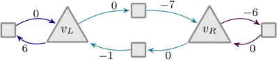
Fig. 3. The weighted game graph(V, E(1))constructed from the graph of Figure 2.
ExampleIII.3. The weighted game graph obtained from the multi-weighted game graph of Example II.1 is depicted in Figure 3 (indeed|V| · kE(2)k+ 1 = 7). Max has a positional
optimal strategy consisting in moving tovL and using the left (blue) loop; every vertex has value 6.
The outcome of this encoding ofd-dimensional weights in
E(1) is the following, easy to establish, proposition.
Proposition III.4. The total weight of a simple cycle in the multi-weighted game graph(V, E, d)is≺0(or=0, or0, respectively) if and only if the total weight of the cycle in the weighted game graph(V, E(1))is negative (or zero, or positive, respectively).
In order to show the positional determinacy of lexicographic energy games, we rely on the following lemma proven in the appendix.
Lemma III.5. If the value of the mean-payoff game
MP(V, E(1)) is non-negative (negative, resp.) at a vertex v,
then by using a positional optimal strategy from that mean-payoff game, Player1(Player2, resp.) wins the corresponding lexicographic energy game LexEn(V, E, d)fromv.
Proof of Theorem III.2. By Lemma III.5, in order to compute a positional winning strategy for one the players in a lexi-cographic energy game LexEn(V, E, d), it suffices to find a positional optimal strategy in the corresponding mean-payoff game MP(V, E(1)). This entails the positional determinacy of lexicographic energy games (cf., e.g., [15]). Regarding complexity, the state-of-the-art algorithm for solving mean-payoff games due to Comin and Rizzi [9] runs in time
O |V|2· |E| · kEk
. Observe that|E(1)|=|E|andkE(1)k=
O|V|d−1·Qd
i=1kE(i)k
, and hence the algorithm of Comin and Rizzi can be used to solve lexicographic energy games in timeO|V|d+1· |E| ·Qd
i=1kE(i)k
.
B. Translation to Lexicographic Energy Games
We now reduce perfect half space games to lexicographic energy games. Given a perfect half space game played on a
d-dimensional multi-weighted game graph, the idea is to play a lexicographic energy game on a2d-dimensional game graph, where the extra dimensions are used to penalise Player2 for changing of perfect half space.
1) Flag Vectors and Interleavings: For anyd-dimensional perfect half spaces H and H0, let the flag vector eH,H0 be
defined for all i = 1, . . . , d by eH,H0(i) = 0def if the i-th
HL vL vR HR
(0,0,0,0) (0,−1,1,1)
(0,0,0,0) (0,−1,1,1)
(0,0,0,−2)
(0,0,0,0) (0,0,0,−2)
[image:6.612.147.465.51.113.2](0,0,0,0)
Fig. 4. The translation of the graph from Figure 2 to lexicographic energy games.
otherwise. For any d-dimensional vectors aandb, leta∆b
be theirinterleaving (a(1),b(1), . . . ,a(d),b(d)).
2) Translation: We write(V ,b E,e 2d)for the weighted game
graph obtained from (V ,b E, db ) by doubling the dimension,
where the even indices of weights in Ee contain the
cor-responding weights from Eb but normalised with respect
to the current perfect half space, and the odd indices are occupied by flag vectors that penalise Player 2for changing the perfect half spaces. More precisely, Ee is the set of all
(v,H)−−−−−−−−−→eH,H0∆(w·H) (v0,H0)such that (v,H)−→w (v0,H0)is inEb.
LetLexEn(V ,b E,e 2d)denote the lexicographic energy game
played on the multi-weighted game graph (V ,b E,e 2d).
Example III.6. We depict in Figure 4 a fragment of the translated game graph (V ,b E,e 2d) for the perfect half space
game from Example II.4. The vertices on the left of the median dashed line are all paired withHL, while those on the right are paired with HR. The flag vectoreHL,HR = (0,1) =eHR,HL
is interleaved with the normalised vectors on the two middle edges entering vR andvL.
In contrast to Example III.1, Player 1 now loses the lexicographic energy game in Figure 4. Indeed, if she plays the middle simple cycle (in cyan) infinitely often, then the energy on the first coordinate converges to0 and the energy in the second coordinate diverges to−∞. Otherwise (i.e., if the number of occurrences of the middle cycle is bounded), the energy in the first three coordinates does not diverge and the energy in the fourth coordinate diverges to−∞.
The correctness of this translation is a direct consequence of the definitions, as shown in the following lemma proven in the appendix.
Lemma III.7. The winning strategies of Playeri,i∈ {1,2}, are the same inPHS(V ,b E, db )andLexEn(V ,b E,e 2d).
Define a strategy τ for Player 2 in the perfect half space gamePHS(V ,b E, db )to be(perfect half space) oblivious atvfor v∈V2 if it chooses the same move in (v,H)for allH. It is
perfect half space obliviousif it is oblivious at all verticesv∈
V2. We are now ready to prove the main theorem of this section.
Theorem III.8. (i) There is an algorithm for solving per-fect half space games whose running time is in
O(3|V| · kEk)2(d+1)3
.
(ii) If Player 2 has a winning strategy in the perfect half space gamePHS(V ,b E, db ), then he has one that is perfect
half space oblivious.
Proof of Theorem III.8(i). The upper bound on the running time is a consequence of Lemma III.7 and Theorem III.2.ii. Observe that the vertex set is of size |Vb| = |V| · |H| ≤ |V| ·(2|V| · kEk+ 1)d2 ≤(3|V| · kEk)d2+1. Regarding the norms,kEek= max{kw·Hk : v
w
−→v0 ∈E,H∈ H}, hence
kEek ≤ d· |V| · kEk 2
≤ (3|V| · kEk)2+logd. Hence a time bound inO((3|V| · kEk)m)where m= (d2+ 1)(2d+ 3) + 2d(2 + logd)≤2(d+ 1)3.
Proof of Theorem III.8(ii). The idea of the following proof is to show that, for any vertex of the weighted game graph winning for Player 2, there is a ‘good’ perfect half spaceH
such that following a positional strategy τH winning from
(v,H)will also win from any(v,H0).
More formally, we prove by induction onk≤ |V2|that there exists a winning positional strategy τ for Player 2 which is perfect half space oblivious atk distinct vertices inV2.
The induction hypothesis obviously holds for k = 0 by using a positional strategy in PHS(V ,b E, db ), which exists by
Theorem III.2 and Lemma III.7. For the induction step, let us suppose thatτ is a winning positional strategy for Player 2
oblivious atk <|V2| distinct verticesv1, . . . , vk∈V2. Let v
be anotherv∈V2 distinct from v1, . . . , vk vertices; τ and v are now fixed for the remainder of the proof.
For all perfect half spaces H, let us denote by τH the strategy τ modified in such a way that it behaves in (v,H0)
as in(v,H)for allH06=H. The result is still a valid strategy (by definition of the perfect half space game) and is of course oblivious atv as well as at v1, . . . , vk. We want to show that
there existsH such thatτH fulfils the induction hypothesis.
This is the case for anyH if v is not in the winning region. We shall therefore assume thatv is in the winning region for Player2; thusτ is winning from every (v,H)but might use different moves depending onH.
a) Good Perfect Half-Spaces: Let us call a perfect half space H good (for τ and v) if τH is winning for Player2
starting in(v,H), and bad otherwise. As shown in the appendix, there must exist a good perfect half space, as otherwise Player2
would not win from v.
Claim III.9. There exists a good perfect half space.
b) A Winning StrategyτH: LetHbe a good perfect half space that exists according to Claim III.9. Let us show thatτH
Player 2. Two cases can happen. Either this play does not visit the vertex v, and in this case it was already a run consistent with τ, and hence it is winning for Player 2. Otherwise it visitsv, and after that point it continues in a way consistent withτH starting from(v,H), and hence is winning for Player2
sinceHis good. This establishes the induction hypothesis, and thus completes the proof of Theorem III.8(ii).
IV. BOUNDINGGAMES
In this section, we define bounding games (as introduced in [12]) and show how these can be reduced to perfect half space games (Theorem IV.2 below). Corollary IV.6 then summarises our knowledge about bounding games.
For a weighted game graph (V, E, d), we denote by
Bnd(V, E, d)the bounding gamein which Player1 (‘Guard’) strives to contain the total weight within somed-dimensional hypercube, while Player2(‘Fugitive’) attempts to escape. More precisely, an infinite play v0
w1
−−→v1
w2
−−→ v2· · · is winning
for Player 1 if and only if the set {kPn
i=1wik : n ∈ N}
of norms of total weights of all finite prefixes of the play is bounded.
ExampleIV.1. Consider again the multi-weighted game graph of Example II.1. Observe that Player1 cannot choose to play solely in the left (blue) cycle, as the accumulated weights would drift towards (+∞,−∞); a similar argument holds with the right (violet) cycle. Hence, she must somehow balance the effect of the two cycles by switching infinitely often between
vLandvR, but the effect of the middle (cyan) cycle then makes the simulated weights drift towards(−∞,−∞). In fact, by the upcoming Theorem IV.2 and as seen in Example II.4, Player2
wins this game.
Theorem IV.2. Let(V, E, d)be a multi-weighted game graph,
v be a vertex inV, andi∈ {1,2}. Playeriwins the bounding game Bnd(V, E, d) from v if and only if Player i wins the perfect half space game PHS(V ,b E, db )fromv.
By Theorem III.8, perfect half space games are determined, hence we can focus on Player2. One implication is straight-forward: a winning strategy for Player 2in PHS(V ,b E, db )also
winsBnd(V, E, d)when ignoring the perfect half spaces. Note that this translates an oblivious strategy in PHS(V ,b E, db ) into
a positional one in Bnd(V, E, d).
Lemma IV.3. If Player2 wins PHS(V ,b E, db )fromv, then he
winsBnd(V, E, d)fromvwith the same strategy (where perfect half spaces are projected away).
Proof sketch. Let Player2 follow a winning strategy for the perfect half space game, projected onto the arena of the bounding game, and consider any resulting play. By the winning condition of the former game, the total weights have unbounded distances from some hyperplane, and so have unbounded norms.
It remains therefore to establish the converse implication in order to complete the proof of Theorem IV.2.
Lemma IV.4. If Player 2wins Bnd(V, E, d)fromv, then he wins PHS(V ,b E, db )fromv.
The proof of this lemma relies on [12, Lemma 5.5]—the most involved result in that paper—, which shows how to construct a winning strategy for Player1fromvinBnd(V, E, d)
from a winning strategy in afirst-cyclevariant FC(V ,b E, db )of PHS(V ,b E, db )fromv. As these first-cycle games are determined,
this entails that, if Player2wins from vin Bnd(V, E, d), then he also wins fromv in the first-cycle game FC(V ,b E, db ), and
it remains to show how to build a winning strategy for him in
PHS(V ,b E, db ). The reasoning itself is surprisingly subtle, and
similar to the one employed in the proof of [12, Lemma 5.3].
Proof of Lemma IV.4. By [12, Lemma 5.5], there exists a winning strategy σ for Player 2 from some (v,H) in the followingfirst-cycle game FC(V ,b E, db ):
1) the game finishes as soon as the play has a suffix C= (v0,H0)
w1
−−→(v1,H1)
w2
−−→ · · · wn
−−→(vn,Hn) such that
v0=vn∈V1;
2) Player2 wins if and only if H0=Hn and C is winning for him: the total weightw(C)=defw1+· · ·+wn of the cycle is in the partially perfect half space defined by the longest common prefix, i.e.w(C)·lcp(C) ≺0 (recall that lcp(C)= lcpdef 1≤i≤nHi).
Let σ∗ denote the strategy for Player 2 from (v,H) in
PHS(V ,b E, db ) that amounts to following σ and repeatedly
cutting out the winning cycles. We want to show thatσ∗is win-ning: consider for this a play(v0,H0)
w1
−−→(v1,H1)
w2
−−→ · · ·
consistent withσ∗ starting fromv0=v.
Let us consider theV1cycle decompositionof this play: the
latter is the infinite sequence of ‘V1-simple’ cyclesCobtained
by pushing the triples of visited vertices and perfect half spaces and indices (v0,H0,0),(v1,H1,1), . . . onto a stack, and as
soon as we push a pair(ve,He, e)with an element(vs,Hs, s) with vs=ve∈V1 already present in the stack, we pop the
cycleCthus formed from the stack and push(ve,He, e)back on top. We call the indicess(C)=defsande(C)=defethestartand end of the cycle, and denote bylcp(C)andw(C)the longest common prefix of its perfect half spaces and total weight respectively. Because σ is winning in FC(V ,b E, db ), all the
cyclesCformed in the cycle decomposition satisfy condition 2 above, henceHs(C)=He(C)andw(C)·lcp(C)≺0.
Let us now consider the longestPsuch that there exists a sufficiently large index iP such that P= lcps(C)≥iP(lcp(C)). We call a partially perfect half space representationHrecurring if H= lcp(C) for infinitely many cycles C in the V1 cycle
decomposition of our play; such a vector H is necessarily non-empty.
Claim IV.5. Pis recurring.
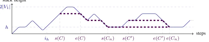
Proof of Claim IV.5. We reason on the height of the stack used to construct the V1 cycle decomposition of the play. Let us
callρi the stack at stepi. Since its height|ρi|is bounded by
stack height
steps
2|V1|
h
[image:8.612.136.482.57.128.2]ih s(C) e(C) s(Cn) s(C0) e(C0)e(Cn)
Fig. 5. Stack heights in the proof of Claim IV.5.
the infinite suffix starting fromih. We depict the stack heights along the play in blue in Figure 5.
Let us call adownward patha sequence of cyclesC1, . . . , Cn such that, for all 1 ≤ i < n, Ci and Ci+1 are either two
successive cycles with |ρs(Ci)|>|ρs(Ci+1)| or two cycles (not
necessarily successive) witheCi =sCi+1. Observe that in both
cases, they visit a common perfect half space HeCi, hence
lcp(Ci)andlcp(Ci+1)are comparable for the prefix ordering.
Assume there are two recurring representations of partially perfect half spacesH andH0. Let us show that they have a common prefix that is also recurring. For this, consider two occurrenceslcp(C) =Handlcp(C0) =H0ofHandH0 with
ih< s(C)< s(C0). As shown by the thick dashed violet line in Figure 5, and since a stack height of h occurs infinitely often, there must be two downward paths C = C1, . . . , Cn resp. C0=Cn+m, . . . , Cn fromC resp.C0 to a single cycle
Cn. Thus the sequence C =C1, . . . , Cn, . . . , Cn+m=C0 is such that, for all1≤i < n+m,lcp(Ci)and lcp(Ci+1)are
comparable for the prefix ordering. The set{lcp(Ci) : 1≤i≤
n+m}is a finite meet-semilattice for the prefix ordering, thus with a bottom element G≤prefH,H0. As there are infinitely
many such pairs of occurrences of the recurringHandH0 and finitely many different such GwithkGk ≤ |V| · kEk, one of the latter must be recurring.
To conclude the proof, assume now thatPis not recurring and let us derive a contradiction. Note that, for all cyclesC
with s(C) ≥ iP, P ≤pref lcp(C). Since P is not recurring,
there must be two incomparable recurring H and H0, such that P<prefH andP<prefH0; we shall further assume that
H is minimal in length with this property. By the previous argument, they have a common prefix G<prefH,H0, which
is also recurring, and which we shall also assume minimal in length. Since H was chosen minimal, there is no recurring
G0 incomparable withG, and sinceGis minimal, there is no recurringG0 <prefGeither, hence there exists an indexisuch thatG= lcps(C)≥i(lcp(C)). AsP≤prefGandPwas chosen of maximal length with this property, P=Gis recurring.
Let us conclude the proof of Lemma IV.4. Write P as
(p1, . . . ,p|P|). For all cycles C with s(C) ≥ iP, P ≤pref
lcp(C)shows thatw(C)·P0. There are then|P|+ 1cases for such cyclesC: either there is1≤k≤ |P|withw(C)·pk<
0 and w(C)·p`= 0for all1≤`≤k, or w(C)·P=0. By Claim IV.5, the|P| first cases occur (cumulatively) infinitely often; letk∗with1≤k∗≤ |P|be the smallest that does. Then, as there are only finitely many occurrences of cases k < k∗,
and finitely manywj andHj not taken into account in the set of cycles C withs(C)≥iP,(p1, . . . ,pk∗)is a witness for
Definition II.3: Player2wins the play.
By Theorem III.8, Theorem IV.2 and the proof of Lemma IV.3, we now have the following improvement over [12, Corollary 3.2].
Corollary IV.6. (i) There is an algorithm for solving bound-ing games whose runnbound-ing time is in(|V| · kEk)O(d3).
(ii) Player2 has positional winning strategies for bounding games.
V. MULTI-DIMENSIONALENERGYPARITYGAMES
In this section, we define multi-dimensional energy parity games (as introduced in [7]) as well as extended multi-dimensional energy games (from [5]), and show how to solve them with an arbitrary (Corollary V.5) or a given (Corollary V.7) initial credit.
A. Multi-Dimensional Energy Parity Games
Themulti-dimensional energy parity gamesare played on finite multi-weighted game graphs (V, E, d)enriched with a priority function π:V → N>0; we let p be the number of
distinct even priorities. Given an initial credit c ∈ Nd, we denote by EnParc(V, E, d, p) the multi-dimensional energy
parity game where Player 1 wins a playv0
w1
−−→v1
w2
−−→v2· · ·
if it satisfies
• theenergy objective: for alli >0, her energy level at step
iis non-negative on all components:c+P
j≤iwj≥0, where comparisons are taken componentwise, and
• the parity objective: the least priorityπ(vi)that appears infinitely often is odd;
Player 2 wins the play otherwise. A multi-dimensional energy game ignores the parity condition—equivalentlyπ(v) = 1for allv∈V.
Example V.1. Let us consider once more the graph of Ex-ample II.1. Player 2 wins the energy game with any initial credit: if Player 1 eventually uses only the left (blue) loop, then the second component will eventually become negative, and similarly for the right (violet) loop and the first component. Hence she must switch infinitely often between her two vertices using the middle (cyan) loop, but this decreases the 1-norm of her current energy level.
3 2 2
4
1
0 0
0 0
−1
[image:9.612.86.263.48.200.2]0
Fig. 6. A1-weighted game graph with priorities.
0,−1,0 0,−1,0
0,0,−1 0,0,0
0,0, ω 0,0,0
−1, ω, ω
0,−1,0
Fig. 7. An extended3-weighted game graph encoding Figure 6.
in this game: due to the energy objective the violet loop on the right can be played at mostc times, and eventually only the cyan loop on the left will be played, but then the parity objective is not satisfied by the play.
B. Extended Multi-Dimensional Energy Games
Extended multi-dimensional energy games allow special weights (denoted by ‘ω’) that let Player1 choose any value she wants for the component. Formally, letZω
def
=Z] {ω}; in
infinity norms of the extended multi-weights,ω is treated as1. An extended (finite) multi-dimensional weighted game graph (V, E, d), whereE⊆(V1×Zdω×V2)∪(V2×Zd×V1). A play on
such a graph is an infinite sequencev0
w1
−−→v1
w2
−−→v2· · · such
thatvi
ui+1
−−−→vi+1∈Efor all0≤iandwi+1instantiatesui+1
by replacing ω’s with values fromN; strategies for Player 1 now have to specify how to instantiate ω’s to form plays. Using the energy objective as before to determine winners of plays, we obtain the extended multi-dimensional energy game
ExtEnc(V, E, d)wherecis the initial credit [5].
The following proposition shows how to get rid of priorities in multi-dimensional energy parity games at the price of extra dimensions and the use of extended games: each even priority is associated with an extra dimension, which is decremented by one upon entering a vertex with this priority, and incremented by ω upon entering a vertex with a smaller odd priority (a pair of additional vertices might need to be introduced if the originating vertex was a Player 2vertex); see Figure 7 for the extended multi-weighted game thus constructed from Figure 6.
Fact V.3(Janˇcar [11, Lemma 1]). Let(V, E, d)be a weighted game graph, v ∈ V an initial vertex, π a priority function with pdistinct even priorities, andc∈ Nd an initial credit. We can construct in logarithmic space an extended weighted game graph(V0, E0, d+p)withV ⊆V0,|V0| ≤3|V|,|E0| ≤ |E|+ 2|V|, andkE0k=kEksuch that:
(i) Player 1 wins EnParc(V, E, d, p) from v if and
only if there exists c0 ∈ Np such that she wins
ExtEncc0(V0, E0, d+p)fromv, and
(ii) Player 2 wins EnParc(V, E, d, p)from v if and only if
for allc0∈Np he winsExtEncc0(V0, E0, d+p)fromv.
−1,0,0 0,0,0
0,0,0 0,0,0
−1,0,0
0,0,0 0,1,0
0,0,0 0,0,1 0,0,0
0,−1,0 0,0,0
[image:9.612.339.538.49.147.2]0,0,−1 0,0,0
Fig. 8. Part of the translation of Figure 7 for bounding games.
C. Arbitrary Initial Credit
We show how extended multi-dimensional energy games, in case the initial credit is existentially quantified for Player 1 (this is the arbitrary initial credit problem), can be solved efficiently by translating them to bounding games. The ideas behind the translation are simple: enable Player 1 to keep the energy bounded at all times by artificial decreasing self-loops, and to instantiateω weights arbitrarily by encoding them as increasing self-loops. However, the proof of correctness (cf. Proposition V.4) is unexpectedly non-trivial and makes use of perfect half space games.
The translation is an extension of the translation in [12, Section 2.3], which did not handleω weights, and performs the following:
• at every vertex owned by Player1 and for every coordi-natei, a self-loop is inserted whose weight is the negative unit vector−ei (these make use of new dummy Player2 vertices, to meet the requirements of player alternation and weight determinacy);
• for every edge whose weight uis not inZd, allω
[image:9.612.94.256.51.95.2]coor-dinates inuare replaced by0, and then a dummy Player 2 vertex is inserted succeeded by a new Player 1 vertex that has a self-loop of weight ei for each coordinate i that wasω inu(the latter make use of further dummy Player2 vertices as before).
Figure 8 illustrates this construction on the right violet loop of the graph of Figure 7.
Proposition V.4. Let (V, E, d) be an extended multi-dimensional weighted game graph andv∈V an initial vertex. We can construct in logarithmic space a multi-dimensional weighted game graph (V†, E†, d) with V ⊆ V†, |V†| ≤ (d+ 1)|V|+ (d+ 2)|E|, |E†| ≤ 2(d+ 1)|E|+ 2d|V|, and
kE†k=kEk such that:
(i) Player 1 winsExtEnc(V, E, d)fromv for somec∈Nd if and only if she wins Bnd(V†, E†, d)fromv, and
(ii) Player 2 winsExtEnc(V, E, d)fromv for allc∈Nd if and only if he winsBnd(V†, E†, d)fromv.
Proof. Regarding the right-to-left implication in item (i), by [12, Lemma 3.1], Player 1 has a winning strategy σ in
Bnd(V†, E†, d)fromv that ensures that all total weights are at mostB= (4def |V†| · kE†k)2(d+2)3
[image:9.612.86.263.125.192.2]By the determinacy of bounding games (cf. Theorem IV.2, Theorem III.8 and Theorem III.2), it now suffices to establish the right-to-left implication in item (ii). Letτbe a winning strat-egy of Player 2 in the perfect half space game PHS(Vc†,Ec†, d),
that is positional and perfect half space oblivious, and letτ be its projection onto the extended graph (V, E, d).
Consider anyc∈Nd, any playπinExtEnc(V, E, d)fromv
that is consistent withτ, and letπc† be a play inPHS(Vc†,Ec†, d)
from v that corresponds toπ(i.e., where the instantiations of
ω weights inπare reproduced by the corresponding increasing self-loops). Observe that any Player 2 vertexv0inπalso occurs in cπ†, and so the perfect half space chosen by τ at v0 must
contain every negative unit vector −ei (otherwise, Player 1 could proceed to win by repeating forever one of the artificial self-loops at the successor of v0), i.e., be disjoint from the non-negative orthantQd
≥0.
Sinceτis winning, there exists a partially perfect half space
(g1, . . . ,gk)which is a prefix of all perfect half spaces that are chosen by τ along a suffix ofcπ†, and there exist a1,b1,
. . . ,ak−1,bk−1 such that:
• the dot products of the total weights along cπ† with gk
are unbounded below, and
• for every `= 1, . . . , k−1, the dot products of the total
weights alongcπ† withg` are in the interval[a`, b`].
Hence, for the sequence of total weights along π with c
subtracted, the same holds. But, by the observation above, the denotation of (g1, . . . ,gk) is disjoint from the non-negative orthant, implying that
{x·gk : c+x≥0and∀1≤` < k,x·g` ∈ [a`, b`]} is bounded below. We conclude that the total weights along π
are not contained in Nd−c, showing as required thatπis a
winning strategy inExtEnc(V, E, d).
From Corollary IV.6, Fact V.3 and Proposition V.4, we obtain our first improved upper bound.
Corollary V.5. The arbitrary initial credit problem for multi-dimensional energy parity games on (V, E, d) with p even priorities is solvable in time(|V| · kEk)O((d+p)3log(d+p)).
We also deduce that Player 2 has positional winning strategies in multi-dimensional energy parity games with arbitrary initial credit; this could already be derived by Fact V.3 from the case of extended energy games with arbitrary initial credit, shown in Lemma 19 in the arXiv version of [5].
D. Given Initial Credit
Thegiven initial credit problemfor multi-dimensional energy parity games takes as input a multi-weighted game graph
(V, E, d), a priority function π, an initial vertex v, and an initial creditcinNd and asks whether Player 1 wins the
multi-dimensional energy parity game EnParc(V, E, d, π)fromv.
Following [12, Lemma 3.4], we show that any multi-dimensional energy parity game with a given initial credit
is equivalent to a bounding game played over a doubly-exponentially larger graph in terms of d, and exponentially larger in terms ofp.
Lemma V.6. be a multi-weighted game graph, π a priority function with pdistinct even priorities, andv∈V. One can construct in timeO(|V‡| · |E|+d·logkck)a multi-weighted game graph (V‡, E‡, d+p) and a vertex vc in V‡, where
|V‡| is in(|V| · kEk)2O(dlog(d+p)) andkE‡k=kEk such that,
for alli∈ {1,2}, Playeri wins the multi-dimensional energy parity gameEnParc(V, E, d, π)fromv if and only if Playeri
wins the bounding gameBnd(V‡, E‡, d+p)fromvc.
Proof sketch. We use the same arguments as in the proof of [12, Lemma 3.4]. The only difference is that we need to handle the parity condition, and thus to go through extended multi-dimensional energy games and replace [12, Proposition 2.2] with the combination of Fact V.3 and Proposition V.4. These only incur a polynomial overhead in the size of the weighted game graphs, hence a bound for|V‡|in(|V| · kEk)2O(d‡logd‡)
withd‡=defd+pcan be deduced directly from [12, Lemma 3.4]. We refine this bound by observing that only the first d
components of the (d+p)-dimensional bounding game we construct should be treated as initialised, while thepremaining ones in Fact V.3 are arbitrary, hence the blowing-up construction of [12, Lemma 3.4] only needs to be applieddtimes, yielding instead a bound in (|V| · kEk)2O(dlogd‡); see Eq. (9) in the
arXiv version of [12].
By applying Corollary IV.6 to the game graph(V‡, E‡, d+p)
and since|E| ≤ |V|2, we obtain a
2-EXPTIMEupper bound on the given initial credit problem, which is again pseudo-polynomial whendandpare fixed.
Corollary V.7. The given initial credit problem with initial creditcfor multi-dimensional energy parity games on(V, E, d) withpeven priorities is solvable in time
(|V| · kEk)2O(d·log(d+p))+O(d·logkck).
This matches the 2-EXPTIME lower bound from [10], and generalises [12, Theorem 3.5] to multi-dimensional energy parity games. Because the given initial credit problem for energy games of fixed dimension d≥4 and number of even prioritiesp= 0is alreadyEXPTIME-hard [10], there is no hope of improving the pseudo-polynomial bound in Corollary V.7 to a polynomial one.
VI. CONCLUDINGREMARKS
In this paper, we have shown a chain of reductions and strategy transfers from multi-dimensional energy parity games to perfect half space games and lexicographic energy games, see Figure 1.
closes complexity gaps for several problems already mentioned in the introduction:
• deciding extended multi-dimensional energy games with given initial input [5],
• deciding whether a Petri net weakly simulates a finite state system, or satisfies a formula of the µ-calculus fragment defined in [1], and
• deciding the model-checking problem for RB±ATL [2].
The second outcome is a rather precise description of the winning strategies for Player 2 in these games. Here, the perfect half space viewpoint is especially enlightening: Player2
can win by ‘announcing’ in which perfect half spaces it is attempting to escape.
APPENDIX
A. Proof of Theorem III.2
Lemma III.5. If the value of the mean-payoff game
MP(V, E(1)) is non-negative (negative, resp.) at a vertex v,
then by using a positional optimal strategy from that mean-payoff game, Player1(Player2, resp.) wins the corresponding lexicographic energy game LexEn(V, E, d)fromv.
Proof. We prove the lemma for Player2(in mean-payoff termi-nology, Min); the argument for Player1(Max) is analogous. For this, let us fix ourselves a positional optimal strategy for Min in the mean-payoff game(V, E(1)). We show that this strategy is also winning for Player 2 in the lexicographic energy game
LexEn(V, E, d). Hence, in the rest of the proof, we consider a playP consistent with this strategy inLexEn(V, E, d), and we aim at showing that it is winning.
Let C1, C2, . . . be the infinite sequence of simple cycles
obtained by the ‘cycle decomposition’ of the playP: we start with an empty sequence of cycles, we then push successive vertices of the play on a stack, and each time we push a vertex that is already present on the stack, we pop the resulting simple cycle from the top of the stack and add it to the sequence of simple cycles. Observe (?) that every simple cycle
C1, C2, . . . has total multi-weight≺0. Indeed, as a cycle in
the strategy subgraph of an optimal strategy for Min in the mean-payoff game MP(V, E(1))with a negative value, it has a negative total weight [15], and hence the observation (?) follows by Proposition III.4.
For a cycle C in the multi-weighted game graph(V, E, d), call the leading dimensionthe least k = 1, . . . , d such that
w(C)(k)6= 0(recall thatw(C)is the total multi-weight of the edges in the cycle). The leading dimensionk∗ of the playP
is the smallest dimension that is the leading dimension of infinitely many cycles C1, C2, . . .; note that in the proof for
Player 1,k∗ can equald+ 1.
The core of the proof is now contained in the following claims A.1 and A.2.
Claim A.1. For all 1≤` < k∗, lim infnP n
i=1w(Ci)(`)<
+∞.
Proof of Claim A.1. Indeed, by the definition of k∗, for all
` < k∗, we have thatw(Ci)(`) = 0for all sufficiently large i.
Hence the sequence of sums Pn
i=1w(Ci)(`) is eventually
constant, so its inferior limit is finite.
Claim A.2. If k∗ ≤ d, then lim supnPn
i=1w(Ci)(k
∗) =
−∞.
Proof of Claim A.2. Indeed, from the definition ofk∗and the fact that every cycle in the decomposition has total weight
≺0, we have that w(Ci)(k∗)is:
• ≤ −1 for infinitely manyi; • ≤0for all sufficiently largei.
The sequence of sums Pn
i=1w(Ci)(k) therefore has limit superior−∞.
From the two above claims, we get that the play P is won by Min. The reader may worry that the expressions of the form ‘Pn
i=1w(Ci)(`)’ differ from those in the definition
of lexicographic energy games: there might be a non-empty simple path remaining indefinitely ‘on the stack’ of the cycle decomposition, and thus not taken into account. However, if we want just to determine whether the corresponding limit inferior (superior, resp.) is less than +∞(equal to −∞, resp.), then the discrepancy is benign because, for every simple pathP0, we have |w(P0)(k)| ≤ |V| · kEk.
B. Proof of Lemma III.7
Lemma III.7. The winning strategies of Playeri,i∈ {1,2}, are the same inPHS(V ,b E, db )and LexEn(V ,b E,e 2d).
Proof. Consider any infinite play
P = (def v1,H1)
w1
−−→(v2,H2)
w2
−−→ · · ·
in the perfect half space game PHS(V ,b E, db ) along with its
corresponding play
e
P = (def v1,H1)
eH1,H2∆(w1·H1)
−−−−−−−−−−−→(v2,H2)
eH2,H3∆(w2·H2)
−−−−−−−−−−−→ · · ·
in the lexicographic energy gameLexEn(V ,b E,e 2d).
We show that P is winning for Player i in PHS(V ,b E, db )
if and only if Pe is winning for the same player in LexEn(V ,b E,e 2d). This in turn entails that winning strategies
for each player can be transferred between the two games. It suffices to show this for Player 2. If Pe is winning
for Player 2, then there exists 1 ≤ k ≤ 2d such that
lim supnPn
j=1(eHj,Hj+1∆wj·Hj)(k) =−∞and for all1≤
` < k,lim infnPnj=1(eHj,Hj+1∆wj·Hj)(`)<+∞. Since
the coefficientseHj,Hj+1 are all non-negative,k cannot
corre-spond to one of these dimensions. Hencekis even; letkˆ=defk/2. Becauselim infnPnj=1(eHj,Hj+1∆wj·Hj)(`)<+∞for all
odd 1≤` < k, we deduce that the visited perfect half spaces
H1,H2, . . . differ on their firstkˆcoordinates only finitely many
times. Hence there is an infinite suffix of the play where all the perfect half spaces share a common prefix(g1, . . . ,gkˆ). Then lim supn
Pn
j=1wj ·gˆk = lim supn
Pn
j=1(eHj,Hj+1 ∆wj ·
Hj)(2ˆk) = −∞and for all 1 ≤` <ˆ ˆk, lim infnP n j=1wj·
gˆ`= lim infnP n
j=1(eHj,Hj+1∆wj·Hj)(2ˆ`)<+∞, hence
Conversely, if P is winning for Player 2 in the perfect half space gamePHS(V ,b E, db ), then there is an infinite suffix
starting at some index i with G lcpj≥iHj satisfying Definition II.3, and let k=def|G|. The kfirst odd coordinates of the weights in the corresponding infinite suffix in Pe
are thus all 0, hence the energy will not diverge on these coordinates. Furthermore, the k first even coordinates in the same suffix are such that lim supn
Pn
j=i(eHj,Hj+1 ∆wj ·
Hj)(2k) = lim supn
Pn
j=iwj · gk = −∞ and, for all
1 ≤ ` < k, lim infnP n
j=i(eHj,Hj+1 ∆ wj · Hj)(2`) =
lim infnP n
j=iwj ·g` < +∞. Thus Pe is also winning for
Player 2 inLexEn(V ,b E,e 2d).
C. Proof of Theorem III.8(ii)
Key Remark: For a strategy τ0 of Player2, we say that a path is (τ0, v)-elementary pathif it is consistent withτ0, it starts in some(v,H), ends in some(v,H0), and does not visit the vertex v in between. Consider a(τ, v)-elementary pathP
starting in(v,H)and ending in(v,H0). Then there is a(τH, v) -elementary pathPH0 that is exactly likeP but for the fact that it begins in(v,H0). This one happens to be acycleconsistent withτH. Then we clearly havelcp(P)≤preflcp(PH0), since
every perfect half space that occurs in PH0 already occurs in
P. Since furthermore w(PH0) =w(P), this means that ifP
is winning for Player 2, then the same holds for PH0.
Claim A.3. If a perfect half spaceH is bad then there exists a (τ, v)-elementary path starting in (v,H) and losing for Player2.
Proof of Claim A.3. Indeed, if H is bad, there exists a play resulting from playing a strategy for Player 1 from (v,H)
againstτH, which is winning for Player 1; by Theorem III.2 and Lemma III.7 we can assume this strategy to be positional. Two cases may happen: Either this play never visitsv (except at the initial position). In this case, this play was already a play consistent withτ, contradicting the fact that the strategyτwas winning from(v,H). Otherwise, the infinite play encounters at least once more some vertex(v,H0). LetP be the prefix of the
play from (v,H)to(v,H0). This is a (τ, v)-elementary path.
SincePhas been obtained from the fight of a positional strategy for Player 1againstτH, the infinite play ultimately repeats the
cyclePH0. ThusPH0 is losing for Player2. According to the
above key remark,P was thus already losing for Player2.
Claim III.9. There exists a good perfect half space.
Proof of Claim III.9. Assume for the sake of contradiction that all perfect half spaces are bad. We shall prove that in this case τ was losing from(v,H). Let us fix for all perfect half spaces H a(τ, v)-elementary pathP(H)starting from(v,H)
ending in some (v, f(H)) and losing for Player 2 (it exists according to Claim A.3). Let us now construct a play consistent withτstarting from(v,H)as follows: assuming the partial play constructed so far ends in(v,H), we extend it by concatenating the pathP(H)to it, yielding a longer play ending in(v, f(H)). We iterate this process and, going to the limit, we obtain an
infinite play P consistent with τ. However, this play is an infinite concatenation of finitely many P(H) paths, which are all losing for Player 2. Hence P is losing for Player 2. This contradicts the fact thatτ was assumed to be winning from (v,H). The claim is proved: there has to be a good perfect half space.
ACKNOWLEDGEMENTS
Work funded in part by the EPSRC grants EP/M011801/1 and EP/P020992/1, and the ERC grant 259454 (GALE). The authors thank Jo¨el Ouaknine and Prakash Panangaden for organising and hosting the Infinite-State Systems workshop at Bellairs Research Institute in March 2015, where this work started.
REFERENCES
[1] P. A. Abdulla, R. Mayr, A. Sangnier, and J. Sproston, “Solving parity games on integer vectors,” in Concur 2013, ser. LNCS, vol. 8052. Springer, 2013, pp. 106–120.
[2] N. Alechina, N. Bulling, S. Demri, and B. Logan, “On the complexity of resource-bounded logics,” inRP 2016, ser. LNCS, vol. 9899. Springer, 2016, pp. 36–50.
[3] N. Alechina, N. Bulling, B. Logan, and H. N. Nguyen, “The virtues of idleness: A decidable fragment of resource agent logic,”Artif. Intell., 2017, to appear.
[4] R. Bloem, K. Chatterjee, T. A. Henzinger, and B. Jobstmann, “Better quality in synthesis through quantitative objectives,” inCAV 2009, ser. LNCS, vol. 5643. Springer, 2009, pp. 140–156.
[5] T. Br´azdil, P. Janˇcar, and A. Kuˇcera, “Reachability games on extended vector addition systems with states,” inICALP 2010, ser. LNCS, vol. 6199. Springer, 2010, pp. 478–489, arXiv version available from http://arxiv.org/abs/1002.2557.
[6] V. Bruy`ere, N. Meunier, and J. Raskin, “Secure equilibria in weighted games,” inCSL-LICS 2014, 2014, pp. 26:1–26:26.
[7] K. Chatterjee, M. Randour, and J.-F. Raskin, “Strategy synthesis for multi-dimensional quantitative objectives,”Acta Inf., vol. 51, no. 3–4, pp. 129–163, 2014.
[8] T. Colcombet and D. Niwi´nski, “Lexicographic energy games,” Manuscript, 2017.
[9] C. Comin and R. Rizzi, “Improved pseudo-polynomial bound for the value problem and optimal strategy synthesis in mean payoff games,” Algorithmica, 2016, to appear.
[10] J. Courtois and S. Schmitz, “Alternating vector addition systems with states,” inMFCS 2014, ser. LNCS, vol. 8634. Springer, 2014, pp. 220–231.
[11] P. Janˇcar, “On reachability-related games on vector addition systems with states,” inRP 2015, ser. LNCS, vol. 9328. Springer, 2015, pp. 50–62.
[12] M. Jurdzi´nski, R. Lazi´c, and S. Schmitz, “Fixed-dimensional energy games are in pseudo-polynomial time,” in ICALP 2015, ser. LNCS, vol. 9135. Springer, 2015, pp. 260–272, arXiv version available from https://arxiv.org/abs/1502.06875.
[13] A. Puri, “Theory of hybrid and discrete systems,” Ph.D. dissertation, University of California, Berkeley, 1995.
[14] Y. Velner, K. Chatterjee, L. Doyen, T. A. Henzinger, A. Rabinovich, and J. Raskin, “The complexity of multi-mean-payoff and multi-energy games,”Inform. and Comput., vol. 241, pp. 177–196, 2015.