Phantom walkabouts in wireless sensor networks

(1)

warwick.ac.uk/lib-publications

Original citation:

Gu, Chen, Bradbury, Matthew S. and Jhumka, Arshad (2017) Phantom walkabouts in wireless

sensor networks. In: 32nd ACM SIGAPP Symposium On Applied Computing, Marrakech,

Morocco, 3-7 April 2017. Published in: Proceedings of the Symposium on Applied Computing

pp. 609-616.

Permanent WRAP URL:

http://wrap.warwick.ac.uk/84296

Copyright and reuse:

The Warwick Research Archive Portal (WRAP) makes this work by researchers of the

University of Warwick available open access under the following conditions. Copyright ©

and all moral rights to the version of the paper presented here belong to the individual

author(s) and/or other copyright owners. To the extent reasonable and practicable the

material made available in WRAP has been checked for eligibility before being made

available.

Copies of full items can be used for personal research or study, educational, or not-for profit

purposes without prior permission or charge. Provided that the authors, title and full

bibliographic details are credited, a hyperlink and/or URL is given for the original metadata

page and the content is not changed in any way.

Publisher’s statement:

© ACM, 2017. This is the author's version of the work. It is posted here by permission of

ACM for your personal use. Not for redistribution. The definitive version was published in

Proceedings of the Symposium on Applied Computing pp. 609-616. (2017)

http://doi.acm.org/10.1145/3019612.3019732

A note on versions:

The version presented here may differ from the published version or, version of record, if

you wish to cite this item you are advised to consult the publisher’s version. Please see the

‘permanent WRAP url’ above for details on accessing the published version and note that

access may require a subscription.

(2)

Phantom Walkabouts in Wireless Sensor Networks

Chen Gu

Department of Computer Science University of Warwick, Coventry

United Kingdom, CV4 7AL [email protected]

Matthew Bradbury

Department of Computer Science

University of Warwick, Coventry United Kingdom, CV4 7AL [email protected]

Arshad Jhumka

Department of Computer Science

University of Warwick, Coventry United Kingdom, CV4 7AL [email protected]

ABSTRACT

As wireless sensor networks (WSNs) have been applied across a spectrum of application domains, the problem of source location privacy (SLP) has emerged as a significant issue, particularly in security-critical situations. In the seminal work on SLP, phantom routing was proposed as a viable approach to address SLP. However, recent work has shown some limitations of phantom routing such as poor perfor-mance with multiple sources. In this paper, we propose

phantom walkabouts, a novel version and more general

ver-sion of phantom routing, which performs phantom routes

of variable lengths. Through extensive simulations we show that phantom walkabouts provides high SLP levels with a low message overhead and hence, low energy usage.

CCS Concepts

•Computer systems organization→Embedded and cyber-physical systems;Sensor networks;

Keywords

Source Location Privacy; Wireless Sensor Networks; Routing; Phantom routing; Phantom walkabouts.

1. INTRODUCTION

A wireless sensor network (WSN) consists of a number of tiny devices, known as sensor nodes or motes, that can sense different attributes of the environment and use radio signals to communicate among themselves. WSNs have enabled the development of many novel applications, including asset monitoring, target tracking and environment control [14] among others, with low levels of intrusiveness. As they are also expected to be deployed in safety and security-critical systems, including military [1] and medical services, the communication protocols used in the WSN must meet the stringent security and privacy requirements.

Threats to privacy in monitoring applications can be con-sidered along two dimensions: (i) content-based threats and

Permission to make digital or hard copies of all or part of this work for personal or classroom use is granted without fee provided that copies are not made or distributed for profit or commercial advantage and that copies bear this notice and the full citation on the first page. Copyrights for components of this work owned by others than the author(s) must be honored. Abstracting with credit is permitted. To copy otherwise, or republish, to post on servers or to redistribute to lists, requires prior specific permission and/or a fee. Request permissions from [email protected].

SAC 2017, April 03 - 07, 2017, Marrakech, Morocco

c

2017 Copyright held by the owner/author(s). Publication rights licensed to ACM. ISBN 978-1-4503-4486-9/17/04. . . $15.00

DOI:http://dx.doi.org/10.1145/3019612.3019732

(ii) context-based threats. Content-based privacy threats re-late to use of the content of the messages broadcast by sensor nodes, such as gaining the ability to read an eavesdropped encrypted message. There has been much research address-ing the issue of providaddress-ing content privacy, e.g., SPINS [18], with most efforts in this area focusing on the use of cryp-tographic techniques. On the other hand, context-based privacy threats focus on the context in which messages are broadcast and how information can be observed or inferred by attackers. Context is a multi-attribute concept that encom-passes situational aspects of broadcast messages, including environmental and temporal information.

It is often desirable for the source of sensed information to be kept private in a WSN. For example, in a military application, a soldier transmitting messages can uninten-tionally disclose its location, even when encryption is used. Another example is during the monitoring of endangered species where poachers may be tempted to infer the location of the animal to capture it. Real world examples include monitoring badgers [4] and the WWF’s Wildlife Crime

Tech-nology Report1, both of which would likely benefit from SLP

being provided. In this paper, the context we focus on is

that ofsource location.

Techniques that protect this source location are said to provide source location privacy (SLP). In each of the pre-viously mentioned scenarios, it is important to ensure that an attacker cannot find or deduce the location of the asset being monitored, whether it is a soldier or an endangered animal. A WSN setup to forward the information collected about an asset would typically consist of the following: (i)

a dedicated node for data collection called asink node, (ii)

node(s) involved in sending information about these assets

calledsource nodes, and (iii) many other nodes in the

net-work used to route/relay messages over multiple hops from the sources to the sink. It has been shown that even a weak attacker such as a distributed eavesdropping attacker can backtrack along message paths through the network to find the source node and capture the asset [9]. Thus, there is a need to develop SLP-aware algorithms.

A number of techniques have been proposed to provide SLP, such as phantom routing using random walks [9], delays [6], dummy data sources [7, 15] and so forth. In general, the objective can be informally stated as the provision of a high level of source location privacy while spending as little energy as possible. In the seminal work on SLP [9], the phantom routing technique was proposed. Phantom routing is a technique where a source initially sends a message along

1

(3)

a random walk (a.k.a. phantom route) of a certain length (typically a few hops). When the message reaches a phantom node at the end of the walk, the phantom node routes the message towards the sink (e.g., by flooding). However, it was recently shown that the phantom routing technique does not scale well under realistic conditions with (i) multiple sources, (ii) increased source rate and (iii) different network configurations [5]. In this paper, we propose a novel, more

generalised technique calledphantom walkabouts, of which

phantom routing is a specific instance. Phantom walkabouts is essentially phantom routes of varying lengths. Through extensive simulations, we show that phantom walkabouts provides state-of-the-art levels of SLP, helping achieve trade-offs between privacy and energy usage.

The main contributions of this paper are:

• We propose phantom walkabouts, a novel and more

general technique than phantom routing, that help achieve a better trade-off between SLP and energy.

• We show, via extensive simulations, the viability of

phantom walkabouts. For example, under certain pa-rameterisation, phantom walkabouts achieves extremely high SLP with acceptable message overhead.

The remainder of this paper is organised as follows: Sec-tion 2 surveys related work in SLP and SecSec-tion 3 presents the models assumed. In Section 4 we present phantom walk-about. The adopted system and simulation approach are outlined in Section 5. Section 6 presents the results of the experiments conducted. Section 7 concludes this paper with a summary of contributions.

2. RELATED WORK

The SLP problem was first posed around 2004 in [16]. Since then, several techniques have been proposed to address SLP. The solution spectrum spans from simple solutions such as the sending of dummy messages [21, 25] to more

sophisticated techniques such as in [7, 12]. All of these

solutions however entail that a set of nodes is selected to send dummy messages. This range from cyclic entrapment [15] to (controlled) flooding of dummy messages [7, 12]. These solutions also handle different types of attackers, though the focus is on local attackers, as in this paper. Perhaps the most significant disadvantage of the described SLP techniques is the volume of messages broadcast to provide SLP. This leads to increased energy consumption and an increased number of collisions, both of which result in a decreased packet delivery ratio. This means that a tradeoff between energy expenditure and privacy must be made [8], making dummy message schemes challenging for many large-scale networks. However, works such as in [3, 6, 13, 19, 20] do not use dummy messages. In particular, [17] and [9] proposed a

two-phase solution calledphantom routing scheme (PRS).

The messages are sent on a directed random walk where the message is either sent towards or away from a certain node in the network, followed by a the chosen routing protocol. A message from the source node would perform a walk through the network to a location and the node would become a

phantom source node. PRS has received a lot of attention

in the literature. On the other hand, the weaknesses as proposed by [22], [19] and [11] for poor SLP are due to the directed random walk reusing the routing path and exposure of direction information. In order to improve the random

walk quality, [23] proposed using location angles to construct the random walk. On the other hand, [24] used a different approach in GROW, by recording neighbours in a bloom filter which informed the choice of the next node to be used in the random walk. However, there is still scope to improve the nodes that are allocated to take part in the directed random walk. In this paper, we propose an alternative approach to better balance the trade-off between energy efficiency and SLP. There are also a range of work on SLP to handle global attackers, but these are outside the scope of the paper.

3. MODELS

In this section, we present the various models that underpin this work.

3.1 Network Model

We assume a wireless sensor network to contain a set of resource-constrained nodes that communicate using a wireless radio. When a node senses the environment, it generates a message and sends the message towards a dedicated node called the sink. There are several potential routing algorithms for message routing in WSNs. We assume all the nodes to be static, i.e., the topology of the network remains the same and the neighbourhoods of all the nodes remain the same over the duration of the network. We do not assume that links are bidirectional, i.e., links may disappear intermittently.

3.2 Attacker Model

We assume a patient adversary model, known as a distributed eavesdropper, introduced in [9]. The attacker initially starts at the sink and we assume the attacker is equipped with the necessary devices to determine the direction a message originated (such as directional antennas). When the attacker overhears a new message, he will move to the location of the immediate sender, i.e., the neighbour that last forwarded the message. This is commensurate with the attacker model used in [2, 5, 7, 8].

4. PHANTOM WALKABOUTS

In the section, we propose a novel SLP routing protocol,

termed asphantom walkabouts, which is a more generic

ver-sion of the so-called phantom routing strategy. Phantom walkabouts is basically phantom routing with variable ran-dom walk lengths, which we will show offer better trade-offs than phantom routing. We first briefly explain the rationale behind the protocol and we then explain the algorithms for forming the short and long random walk, the biased long random walk and the overall phantom walkabouts algorithm.

4.1 Overview

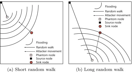
Figure 1a shows the typical scenario during an execution of phantom routing where the source sends a message to a phantom node which lies somewhere between itself and the sink. When the phantom node floods the message to the sink, the first movement of the attacker is towards the phantom node. However, it would be beneficial to have the first movements of the attacker to be away from the source, as shown in Figure 1b. To achieve this, a longer random walk can be used, where the length of the walk exceeds the source-sink distance.

(4)

[image:4.612.332.539.55.126.2]

Table 1: Commonly used notations

Notation Meaning

rwDir Message random walk direction

dir Message random walk direction set

newDir Message new random walk direction

hwalk Message random walk hop-count remaining

δ Message biased random walk direction

α Biased random walk factor

tt Flooding time taken

sp Phantom walkabouts safety period

Ms Short random walk message

Ml Long random walk message

a greater number of nodes for forwarding messages, thus consuming more energy. In that sense, there is a trade-off to be made between the level of SLP gained and the additional amount of energy consumed or message overhead.

As such, we conjecture that phantom walkabouts with a mix of short and long random walk will achieve a higher level of SLP than phantom routing with a bounded message overhead. We denote a phantom walkabouts parametrisation

by P W(s, l), where s, l denote the number of short and

long random walk respectively to be performed in a cycle.

P W(1,1) denotes a repeating sequence of 1 short random

walk followed by 1 long random walk. Phantom routing with

short random walks is denoted byP W(1,0) where there are

no long random walks, and vice versa forP W(0,1). Later,

in this paper, we investigate the SLP levels, and associated

[image:4.612.57.295.73.214.2]

message overhead ofP W(1,0),P W(1,1) andP W(0,1).

Table 1 summarises the most commonly used notations in the paper.

Source node Phantom node Flooding Random walk Attacker movement

Sink node

(a) Short random walk

Source node Phantom node Flooding Random walk Attacker movement

Sink node

(b) Long random walk

Figure 1: Short and long random walk routing examples

4.2 Short Random Walk Routing

Rather than divide node neighbours into two sets (as phan-tom routing does) and thus limit the possible random walk direction, we introduce short random walk routing algorithm that always splits node neighbours into four sets, which in-creases random walk directions, and hence improves short random walk reliability. When the short random walk length

sis less than the source-sink distance, the short random

route is allocated using Algorithm 1 and described below:

• Each node maintains four sets for all its neighbours,

[image:4.612.326.554.162.285.2]

Sn,Ss,SwandSerepresenting four different directions:

Figure 2: Neighbour division example

Algorithm 1Short Random Walk

1: procedureShorRandomWalk(msg,s)

2: N extLocation← ⊥

3: msg.hwalk←s

4: whilemsg.hwalk6= 0do

5: msg.dir←ChooseOneSet(msg)

6: if msg.dir.h6=⊥ ∧msg.dir.v6=⊥then

7: N extLocation←ChooseOne(msg.dir)

8: msg.hwalk←msg.hwalk−1

9: msg.CurrentLocation←N extLocation

10: ForwardMessage(msg.CurrentLocation)

11: Flooding()

north, south, west and east neighbours of a node it-self. This partition can be achieved by landmark nodes

flooding messages during the deployment phase2. After

neighbour nodes partition, the message’s random walk direction presents in two sets, one set for each dimen-sion. The random walk direction has one of four moving

directions, i.e.,dir={h, v}where (h, v)∈ {(Sw, Sn),

(Se, Sn),(Sw, Ss),(Se, Ss)}. For instance, as shown in

Figure 2, a source node randomly choosesSwandSn

directions, i.e.,dir={Sw, Sn}.

• At the beginning of random walk phase, a message

randomly chooses a walk directionrwDir∈dir and

always randomly chooses walk direction fromdirduring

the random walk phase.

• When a message travelledshops (assume random walk

length iss), it has finished the random walk phase. The

message then flood throughout the network so that it reaches the sink node.

4.3 Long Random Walk Routing

Long random walk routing is named as such because the

lengthl is larger than the source-sink distance. It is more

complex than short random walk routing because the message may reach the borderline of the network and the border node cannot forward the message to the previous selected direction.

In this case, we say that the random walk isblocked. If this

happens, the message may not continue to walk along with the previous direction and a new direction is used for the rest random walk. Here we describe a new algorithm for it which is also shown in Algorithm 2.

• Similar to short random walk routing, each node

main-tains four sets for all its neighbours,Sn, Ss, Sw,Se.

Also the node classifies their neighbours into two sets

2

[image:4.612.58.291.429.556.2]

(5)

Algorithm 2Long Random Walk

1: procedureLongRandomWalk(msg,l)

3: msg.hwalk←l

5: msg.dir←ChooseOneSet(msg)

6: ifmsg.dir.h6=⊥ ∧msg.dir.v6=⊥then

7: N extLocation←ChooseOne(msg.dir)

8: else

9: msg.newDir←GetCloserSinkSet()

10: ifmsg.newDir6=⊥then

11: N extLocation←ChooseOne(msg.newDir)

12: else if msg.newDir=⊥ ∧msg.dir=⊥then

13: hwalk←0

14: break

15: else

16: N extLocation←ChooseDirection(msg.dir)

20: Flooding()

by the node-sink distance. If its neighbour nodes have larger node-sink distance than itself, the neighbour

nodes will be classified into theF urtherSinkSet.

Oth-erwise, they will be classified into theCloserSinkSet.

• Now the message holdingrwDiris walking through the

network. IfrwDiris empty, we believe the message is

blocked. In this case,dirbecomesCloserSinkSetand

new direction newDirwill be assigned to one in the

CloserSinkSet. In certain extreme situation whendir

is ∅, the long random walk terminates and the node

become the phantom node. Because we believe the phantom node is farthest from the real source node and ensures the safety of source node that its location will be hard to track.

• Similar to short random walk routing, the flooding

phase will start once the long random walk ends.

4.4 Biased Long Random Walk Routing

A long random walk routing ensures that phantom nodes are far away from the real source node. However, there is a weakness that needs to be addressed for certain topologies. Specifically, consider the topology where the source node lies in the corner of a grid and the sink node in the middle area of the network. As the source locates in the corner, messages will be always transmitted towards the sink node. Owing to the random nature of the walk, the long random walk may “go through” the sink node. In this case, the attacker will notice the message and will move towards the source node, increasing the chance of a source capture.

To address this issue, we develop a biased long random

walk, for the specific topology so as to avoid the case where

the random walk goes close to the attacker. The biased long random walk is described as follow and shown in Algorithm 3.

• The message firstly chooses the biased random walk

direction δ (follow horizontal directionH or vertical

directionV), i.e.,δ∈ {H, V}. If chosen, the message

will continue use the selected biased direction until random walk phase finish or reach the end of that direction.

Algorithm 3Biased Long Random Walk

1: procedureBiasedLongRandomWalk(msg,l)

3: biasedSet← {H, V}

4: msg.hwalk←l

5: msg.biasedDir←ChooseOneDirection(biasedSet)

7: p←GenerateRandomNumber(0,1)

8: if p≤αthen

9: N extLocation←msg.biasedDir

10: ifN extLocation=⊥then

11: N extLocation←biasedSet\ {msg.biasedDir}

12: else

13: N extLocation←biasedSet\ {msg.biasedDir}

14: if N extLocation=⊥then

15: hwalk←0

16: break

20: Flooding()

• A random value θ ∈ [0,1] is generated. We set α

in our experiments to make sure a message has high

probability walking alongδ. Normally the value ofαis

often set larger than 0.5 but less than 1. For instance, if

αis set to 0.8, it indicates the message has nearly 80%

probability transmitting along the previous directionδ.

The node decides to send this message to the neighbour node by following equation:

f(δ, θ, α) =







δ ifθ∈[0, α]

{H, V} \ {δ} otherwise

(1)

• Whenδis blocked, it indicates that the message reach

the end of this direction. Message will choosenewDir∈

{H, V} \ {δ}to continue the random walk until random

walk finishes. IfnewDiris∅, the random walk stops.

Then the flooding phase starts.

4.5 Phantom Walkabouts

In this section, we formalize the phantom walkabouts tech-nique, which extends the phantom routing protocol by adopt-ing variable lengths of phantom routadopt-ing. When a source node

routes a messageM using phantom walkabouts, a decision is

needed regarding whetherMgoes on a short or long random

walk route. The sequencing of messages looks like as follows:

Ms,· · ·, Ms,

| {z }

m

Ml,· · ·, Ml,

| {z }

n

Ms,· · ·, Ms,

| {z }

m

Ml,· · ·, Ml,

| {z }

n

· · ·

Therefore, we observe that the phantom walkabouts consists

ofmmessages on short random walk andnmessages on long

random walk, before the cycle is repeated. Thus,P W(1,1)

(6)

Algorithm 4Phantom Walkabouts

1: procedurePhantomWalkabouts(msg,s,l,P W(m, n))

2: m0_{, n}0_←_{m, n}

3: whileT ruedo

4: ifm0_>₀_then

5: GenerateMessage()

6: ShortRandomWalk(msg, s)

7: m0 ←m0−1

8: else if m0= 0∧n0>0then

9: GenerateMessage()

10: BiasedLongRandomWalk(msg, l)

11: n0_←_n0₋₁

12: else

13: m0_{, n}0_←_{m, n}

4.6 Problem Statement

The problem we address is: Given a source node, a sink, a pair

(s, l) for the short and long random walks length, analyse the

impact on SLP and associated message overhead of various parameterisation on phantom walkabouts. The analysis will capture the trade-offs that can be made regarding levels of SLP and message overhead.

5. EXPERIMENTAL SETUP

In this section we describe the simulation environment, source selection, attacker model and safety period calculation that were used to generate the results presented in Section 6.

5.1 Simulator and Network Configuration

The TOSSIM (V2.1.2) simulation environment was used in all experiments [10]. TOSSIM is a discrete event simulator capable of accurately modelling sensor nodes and the modes of communications between them.

A square grid network layout of sizen×nwas used in

all experiments, with n ∈ {11,15,21,25}, i.e., networks

with 121, 225, 441 and 625 nodes respectively. The node neighbourhoods were generating using an ideal radio model where each node is connected to their north, south, east and west neighbour (if present). Nodes were located 4.5 meters apart. Noise models were created using the first 1000 lines ofmeyer-heavy.txt3. All the nodes are stationary.

Multiple source nodes generated messages and a single sink node collected messages. The set of experiments for each network size were performed with the source node(s) in the corner, and the sink in the centre in the network. The rate at which messages from the real sources was generated was set to be either 1, 2, 4 and 8 messages per second. The source period was normalised with respect to the number of sources so that any configuration will have the same overall message rate. At least 500 repeats were performed for each combination of source location and parameters.

5.2 Source Selection

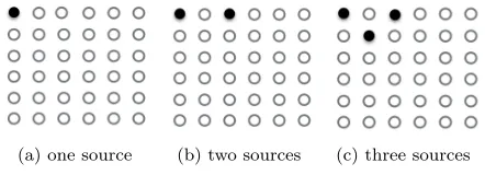
The three source positions we use in our simulations are shown in Figure 3. The reason why the sources are clustered together is because we envision providing SLP for several sensors detecting an asset. Such configurations have previ-ously been shown to provide poor performance [5], hence our focus on trying to provide SLP for this degenarate case.

3_{meyer-heavy.txt is a noise sample file provided with}

TOSSIM.

[image:6.612.327.548.55.135.2]

(a) one source (b) two sources (c) three sources

Figure 3: Network Layouts with Varying Number of Sources

5.3 Safety Period

A metric calledsafety period (which we calltime-to-capture

from here) was introduced in [9] which is the number of messages sent before an attacker captures the source. The higher the time-to-capture is, the higher the source location privacy level. Using the time-to-capture metric means that simulation runtime is unbounded and potentially very large. We thus use an alternative, but analogous, definition for safety period: for each network size, source rate and config-uration, we obtain the time-to-capture when protectionless flooding is used as the routing protocol. Flooding is used as it has been argued to provide the least SLP level, hence any SLP improvement is due to the SLP-aware technique [9]. The safety period is then obtained by increasing this value to account for the attacker potentially making bad moves.

Thus, we calculate the safety period sp as the following,

wherett is the time-to-capture for protectionless flooding.

This definitition is commensurate with [7, 8], but uses a different multiplicative factor due to the difference in the type of SLP technique being used. Intuitively, the safety period captures the time period during which the asset will be at the same location.

sp= 1.3×tt (2)

5.4 Simulation and Parameter Setup

An experiment is made of a single execution of the simulation environment using a specified protocol configuration, network size and safety period. An experiment terminated when any source node had been captured by an attacker during the safety period or the safety period had expired. We will anal-yse two metrics calculated from the simulation experiments

which are now described. Message sent is defined as the

number of messages sent from each source during the experi-ment, the final result is obtained by averaging the number of messages sent over all repeats for a specific parameter

combination. We also define a metric called capture ratio

which is the number of experiments ending in a capture di-vided by the total number of repeats for a specific parameter combination.

In Subsection 4.4, we introduced parameter α used to

implement biased random walk. The larger the value of

α is, the bigger is the chance that the phantom walk will

avoid walking close to the sink. In the simulation, we set

this value to 0.9. When choosing the length of the long and

short random walks, a variety of parameter combinations were considered. Our experiments set the short random

walk seriesS={2,3, . . . ,0.5×ssd}, and long random walk

series L={2 +ssd, . . . ,1.5×ssd}, where ssd is the sink

source distance. The phantom walkabouts combines the short and long random walks such that the following length

(7)

6. RESULTS

6.1 PW(1,0): SLP using Short Random Walks

SLP:In this section, we first establish the base case against

which subsequent improvements will be evaluated. In pre-vious works on phantom routing, the length of the random walk has typically been small, less than the source to sink

distance, which can be represented asP W(1,0), showing the

generality of our framework. Figure 4a contains the results for phantom routing. Two important observations are made:

• The level of SLP increases (i.e., capture ratio decreases)

with increasing message rate. This is counter intuitive in the sense that it can be expected that the capture ratio to be higher as more messages are sent by the nodes and can be captured by the attacker. However, the higher number of messages lead to a much lower safety period, meaning that it is difficult for an attacker to capture the source within the safety period.

• The level of SLP increases with increasing number of

sources, for similar reasons as earlier.

Messages:A high level of SLP can be provided albeit at the expense of a high number of messages (hence, high energy usage). Thus, there is a trade-off to be made between the level of SLP provided and the number of messages transmit-ted [8]. In Figure 5a, we observe that the number of messages increases with increasing network size. It can also be ob-served that the number of messages transmitted is similar at various message rates. However, the number of messages transmitted gets smaller with increasing number of sources. This is due to the fact that the smaller safety period limits the number of messages that can be transmitted.

6.2 PW(1,1): SLP using Alternating Short and

Long Random Walks

As has been shown, phantom routing with smaller random walk yields lower SLP levels but with better message com-plexity while phantom routing with longer random walks yield much better SLP with a higher message overhead. To try and achieve a trade-off between those two factors, we consider the case where a short and a long random walk is

chosen alternately, yielding what we have termed asphantom

walkabouts.

As can be observed from Figures 4a and 4b, alternating between a short and a long random walk in phantom walk-abouts yields, in general, a higher level of SLP than when using short random walks during phantom routing, especially for the larger-sized networks. We conjecture that this phe-nomenon happens due to the fact that the time taken for the message to reach the attacker from a long random walk is comparable to the time taken when time period of message generation and the message reaching an attacker using a short random walk, i.e., due to the longer time for a message to reach an attacker through the longer random walk, an at-tacker may see consecutive messages through shorter random walks. However, this is an area for further investigation.

Further, this improvement comes about with the expected additional message overhead (see Figures 5a and 5b) from the base case. Comparing with the case of having only long random walks during phantom routing, we observe that there is the expected decrease in SLP levels (Figures 4c and 4b) but also in message overheads (Figures 5c and 5b).

6.3 PW(0,1): SLP using Long Random Walks

As explained earlier in Figure 1, we hypothesised that a short random walk will initially drag the attacker towards the source while a longer random walk will drag the attacker away from the source, thereby possibly increasing the SLP levels but also energy usage. In this section, we seek to determine whether the hypotheses hold.

As can be observed from Figures 4a and 4c, the level of SLP provided with a longer random walk is much higher than that with a shorter random walk, thereby corroborating our hypothesis. On the other hand, though the number of messages sent with long random walks is greater than with short random walks (see Figures 5a and 5c), the increase is only nominal, around 15%, while the drop in capture ratio is around a factor of 40. This shows that phantom routing, with a long random walk, offers a much higher level of SLP at the expense of a small increase in message transmissions (i.e., energy expenditure).

7. CONCLUSION

In this paper, we have proposed a novel technique called phantom walkabouts, which extends the phantom routing, to provide a better level of SLP but at lower additional message overhead. Through simulations, we have shown that phantom walkabouts provide much better levels of SLP at certain parameterisation, albeit at only a small message overhead over phantom routing, than phantom routing (PW(1,0)).

References

[1] I. Akyildiz, W. Su, Y. Sankarasubramaniam, and

E. Cayirci. Wireless sensor networks: a survey.

Com-puter Networks, 38(4):393 – 422, 2002.

[2] M. Bradbury, M. Leeke, and A. Jhumka. A dynamic fake source algorithm for source location privacy in

wireless sensor networks. In14th IEEE International

Conference on Trust, Security and Privacy in Computing

and Communications, pages 531–538, August 2015.

[3] C. Chow, M. Mokbel, and T. He. A privacy-preserving location monitoring system for wireless sensor networks. Mobile Computing, IEEE Transactions on, 10(1):94–107, Jan 2011.

[4] V. Dyo, S. A. Ellwood, D. W. Macdonald, A. Markham,

N. Trigoni, R. Wohlers, C. Mascolo, B. P´asztor, S.

Scel-lato, and K. Yousef. Wildsensing: Design and deploy-ment of a sustainable sensor network for wildlife

moni-toring. ACM Trans. Sen. Netw., 8(4):29:1–29:33, Sept.

2012.

[5] C. Gu, M. Bradbury, A. Jhumka, and M. Leeke. As-sessing the performance of phantom routing on source

location privacy in wireless sensor networks. In 2015

IEEE 21st Pacific Rim International Symposium on

De-pendable Computing (PRDC), pages 99–108, Nov 2015.

[6] X. Hong, P. Wang, J. Kong, Q. Zheng, and jun Liu. Effective probabilistic approach protecting sensor traffic.

In Military Communications Conference, 2005.

MIL-COM 2005. IEEE, pages 169–175 Vol. 1, Oct 2005.

(8)

0 10 20 30 40 50

11 15 21 25

Capture Ratio (%)

Network Size

Source Period 0.125 seconds Source Period 0.25 seconds Source Period 0.5 seconds Source Period 1.0 seconds

0 10 20 30 40 50

11 15 21 25

Capture Ratio (%)

Network Size

0 10 20 30 40 50

11 15 21 25

Capture Ratio (%)

Network Size

(a)P W(1,0): Usingshortrandom walks with 1, 2, and 3 source nodes

0 10 20 30 40 50

11 15 21 25

Capture Ratio (%)

Network Size

0 10 20 30 40 50

11 15 21 25

Capture Ratio (%)

Network Size

0 10 20 30 40 50

11 15 21 25

Capture Ratio (%)

Network Size

(b)P W(1,1): Usingalternating short and longrandom walks with 1, 2 and 3 source nodes

0 10 20 30 40 50

11 15 21 25

Capture Ratio (%)

Network Size

0 10 20 30 40 50

11 15 21 25

Capture Ratio (%)

Network Size

0 10 20 30 40 50

11 15 21 25

Capture Ratio (%)

Network Size

[image:8.612.54.559.49.420.2]

(c)P W(0,1): Usinglongrandom walks with 1, 2 and 3 source nodes

Figure 4: SLP level provided by 4 variants of the Phantom Walkabouts algorithm for 1, 2 and 3 sources respectively

Concurrency and Computation: Practice and Experience,

27(12):2999–3020, 2015.

[8] A. Jhumka, M. Leeke, and S. Shrestha. On the use of fake sources for source location privacy: Trade-offs

between energy and privacy. The Computer Journal,

54(6):860–874, 2011.

[9] P. Kamat, Y. Zhang, W. Trappe, and C. Ozturk. En-hancing source-location privacy in sensor network

rout-ing. In 25th IEEE International Conference on

Dis-tributed Computing Systems, 2005. ICDCS 2005. Pro-ceedings., pages 599–608, June 2005.

[10] P. Levis, N. Lee, M. Welsh, and D. Culler. Tossim: accu-rate and scalable simulation of entire tinyos applications.

In Proceedings of the 1st international conference on

Embedded networked sensor systems, SenSys ’03, pages

126–137, New York, NY, USA, 2003. ACM.

[11] L. Lightfoot, Y. Li, and J. Ren. Preserving source-location privacy in wireless sensor network using star

routing. In Global Telecommunications Conference

(GLOBECOM 2010), 2010 IEEE, pages 1–5, Dec. 2010.

[12] J. Long, M. Dong, K. Ota, and A. Liu. Achieving

source location privacy and network lifetime maximiza-tion through tree-based diversionary routing in wireless

sensor networks. Access, IEEE, 2:633–651, 2014.

[13] X. Luo, X. Ji, and M.-S. Park. Location privacy against traffic analysis attacks in wireless sensor networks. In Information Science and Applications (ICISA), 2010 International Conference on, pages 1–6, April 2010.

[14] A. Mainwaring, J. Polastre, R. Szewczyk, and D. Culler. Wireless sensor networks for habitat monitoring. In Proceedings of the First ACM International Workshop

on Wireless Sensor Networks and Applications, 2002.

[15] Y. Ouyang, Z. Le, G. Chen, J. Ford, and F. Makedon. Entrapping adversaries for source protection in sensor

networks. InWorld of Wireless, Mobile and Multimedia

Networks(WoWMoM) 2006., pages 10–34, 2006.

[16] C. Ozturk, Y. Zhang, and W. Trappe. Source-location privacy in energy-constrained sensor network routing.

In Proceedings of the 2nd _{ACM workshop on Security}

of ad hoc and sensor networks, SASN ’04, pages 88–93,

New York, NY, USA, 2004. ACM.

[17] C. Ozturk, Y. Zhang, W. Trappe, and M. Ott. Source-location privacy for networks of energy-constrained

sen-sors. InSoftware Technologies for Future Embedded and

Ubiquitous Systems, 2004. Proceedings. Second IEEE

(9)

0 5000 10000 15000 20000

11 15 21 25

T

otal Messages Sent

Network Size Source Period 0.125 seconds

Source Period 0.25 seconds Source Period 0.5 seconds Source Period 1.0 seconds

0 5000 10000 15000 20000

11 15 21 25

T

otal Messages Sent

0 5000 10000 15000 20000

11 15 21 25

T

otal Messages Sent

(a)P W(1,0): Usingshortrandom walks with 1, 2 and 3 source nodes

0 5000 10000 15000 20000

11 15 21 25

T

otal Messages Sent

0 5000 10000 15000 20000

11 15 21 25

T

otal Messages Sent

0 5000 10000 15000 20000

11 15 21 25

T

otal Messages Sent

(b)P W(1,1): Usingalternating short and longrandom walks with 1, 2 and 3 source nodes

0 5000 10000 15000 20000

11 15 21 25

T

otal Messages Sent

0 5000 10000 15000 20000

11 15 21 25

T

otal Messages Sent

0 5000 10000 15000 20000

11 15 21 25

T

otal Messages Sent

[image:9.612.52.560.48.416.2]

(c)P W(0,1): Usinglongrandom walks with 1, 2 and 3 source nodes

Figure 5: Messages Sent by 4 variants of the Phantom Walkabouts algorithm for 1, 2 and 3 sources respectively

[18] A. Perrig, R. Szewczyk, J. D. Tygar, V. Wen, and D. E. Culler. Spins: Security protocols for sensor networks. Wirel. Netw., 8(5):521–534, Sept. 2002.

[19] R. A. Shaikh, H. Jameel, B. J. D’Auriol, H. Lee, S. Lee, and Y.-J. Song. Achieving network level privacy in

wire-less sensor networks. Sensors, 10(3):1447–1472, 2010.

[20] M. Shao, W. Hu, S. Zhu, G. Cao, S. Krishnamurth, and T. La Porta. Cross-layer enhanced source location

privacy in sensor networks. InSensor, Mesh and Ad

Hoc Communications and Networks, 2009. SECON ’09. 6th Annual IEEE Communications Society Conference

on, pages 1–9, June 2009.

[21] M. Shao, Y. Yang, S. Zhu, and G. Cao. Towards sta-tistically strong source anonymity for sensor networks.

InINFOCOM 2008. The 27th Conference on Computer

Communications. IEEE, April 2008.

[22] H. Wang, B. Sheng, and Q. Li. Privacy-aware routing in

sensor networks. Computer Networks, 53(9):1512–1529,

2009.

[23] W. Wei-Ping, C. Liang, and W. Jian-xin. A source-location privacy protocol in WSN based on source-locational

angle. InIEEE International Conference on

Communi-cations, pages 1630–1634, May 2008.

[24] Y. Xi, L. Schwiebert, and W. Shi. Preserving source location privacy in monitoring-based wireless sensor

networks. InParallel and Distributed Processing

Sym-posium, 2006. IPDPS 2006. 20th International, pages 8 pp.–, Apr. 2006.

[25] Y. Yang, M. Shao, S. Zhu, B. Urgaonkar, and G. Cao. Towards event source unobservability with minimum

network traffic in sensor networks. InProceedings of the

First ACM Conference on Wireless Network Security,