Bayesian Document Generative Model with Explicit Multiple Topics

Proceedings of the 2007 Joint Conference on Empirical Methods in Natural Language Processing and Computational

Bayesian Document Generative Model with Explicit Multiple Topics

Issei Sato

Graduate School of Information Science and Technology,

The University of Tokyo

[email protected]

Hiroshi Nakagawa Information Technology Center,

The University of Tokyo

[email protected]

Abstract

In this paper, we proposed a novel prob-abilistic generative model to deal with ex-plicit multiple-topic documents: Parametric Dirichlet Mixture Model(PDMM). PDMM is an expansion of an existing probabilis-tic generative model: Parametric Mixture Model(PMM) by hierarchical Bayes model. PMM models multiple-topic documents by mixing model parameters of each single topic with an equal mixture ratio. PDMM models multiple-topic documents by mix-ing model parameters of each smix-ingle topic with mixture ratio following Dirichlet dis-tribution. We evaluate PDMM and PMM by comparing F-measures using MEDLINE corpus. The evaluation showed that PDMM is more effective than PMM.

1 Introduction

Documents, such as those seen on Wikipedia and Folksonomy, have tended to be assigned with ex-plicit multiple topics. In this situation, it is impor-tant to analyze a linguistic relationship between doc-uments and the assigned multiple topics . We at-tempt to model this relationship with a probabilistic generative model. A probabilistic generative model for documents with multiple topics is a probability model of the process of generating documents with multiple topics. By focusing on modeling the gener-ation process of documents and the assigned multi-ple topics, we can extract specific properties of doc-uments and the assigned multiple topics. The model

can also be applied to a wide range of applications such as automatic categorization for multiple topics, keyword extraction and measuring document simi-larity, for example.

A probabilistic generative model for documents with multiple topics is categorized into the following two models. One model assumes a topic as a latent topic. We call this model the latent-topic model. The other model assumes a topic as an explicit topic. We call this model the explicit-topic model.

In a latent-topic model, a latent topic indicates not a concrete topic but an underlying implicit topic of documents. Obviously this model uses an unsupervised learning algorithm. Representa-tive examples of this kind of model are Latent Dirichlet Allocation(LDA)(D.M.Blei et al., 2001; D.M.Blei et al., 2003) and Hierarchical Dirichlet Process(HDP)(Y.W.Teh et al., 2003).

In an explicit-topic model, an explicit topic indi-cates a concrete topic such as economy or sports, for example. A learning algorithm for this model is a supervised learning algorithm. That is, an explicit topic model learns model parameter using a training data set of tuples such as (documents, topics). Rep-resentative examples of this model are Parametric Mixture Models(PMM1 and PMM2)(Ueda, N. and Saito, K., 2002a; Ueda, N. and Saito, K., 2002b). In the remainder of this paper, PMM indicates PMM1 because PMM1 is more effective than PMM2.

In this paper, we focus on the explicit topic model. In particular, we propose a novel model that is based on PMM but fundamentally improved.

The remaining part of this paper is organized as follows. Sections 2 explains terminology used in the

following sections. Section 3 explains PMM that is most directly related to our work. Section 4 points out the problem of PMM and introduces our new model. Section 5 evaluates our new model. Section 6 summarizes our work.

2 Terminology

This section explains terminology used in this paper. Kis the number of explicit topics. V is the number of words in the vocabulary. V = {1,2,· · ·, V}is a set of vocabulary index. Y ={1,2,· · · , K}is a set of topic index. N is the number of words in a document.w= (w1, w2,· · · , wN)is a sequence of

N words wherewndenotes thenth word in the

se-quence. wis a document itself and is called words vector. x = (x1, x2,· · ·, xV)is a word-frequency

vector, that is, BOW(Bag Of Words) representation where xv denotes the frequency of word v. wvn

takes a value of 1(0) when wn is v ∈ V (is not

v ∈ V). y = (y1, y2,· · ·, yK) is a topic vector

into which a document w is categorized, whereyi

takes a value of 1(0) when theith topic is (not) as-signed with a documentw. Iy ⊂Y is a set of topic

index i, where yi takes a value of 1 in y. P_i∈Iy

and Πi∈Iy denote the sum and product for all iin

Iy, respectively. Γ(x) is the Gamma function and

Ψis the Psi function(Minka, 2002). A probabilistic generative model for documents with multiple top-ics models a probability of generating a documentw in multiple topicsyusing model parameterΘ, i.e., modelsP(w|y,Θ). A multiple categorization prob-lem is to estimate multiple topicsy∗ of a document w∗ whose topics are unknown. The model parame-ters are learned by documentsD={(wd, yd)}Md=1,

whereM is the number of documents.

3 Parametric Mixture Model

In this section, we briefly explain Parametric Mix-ture Model(PMM)(Ueda, N. and Saito, K., 2002a; Ueda, N. and Saito, K., 2002b).

3.1 Overview

PMM models multiple-topic documents by mixing model parameters of each single topic with an equal mixture ratio, where the model parameterθivis the

probability that word v is generated from topic i. This is because it is impractical to use model

param-eter corresponding to multiple topics whose num-ber is2K _{−1(all combination ofK topics). PMM}

achieved more useful results than machine learn-ing methods such as Naive Bayes, SVM, K-NN and Neural Networks (Ueda, N. and Saito, K., 2002a; Ueda, N. and Saito, K., 2002b).

3.2 Formulation

PMM employs a BOW representation and is formu-lated as follows.

P(w|y, θ) = ΠV

v=1(ϕ(v,y, θ))xv (1)

θ is a K × V matrix whose element is θiv =

P(v|yi = 1).ϕ(v,y, θ)is the probability that word

v is generated from multiple topics y and is de-fined as the linear sum ofhi(y) andθivas follows:

ϕ(v,y, θ) =PK

i=1hi(y)θiv

hi(y) is a mixture ratio corresponding to topici

and is formulated as follows: hi(y) = PKyi

j=1yj,

PK

i=1hi(y) = 1.

(ifyi = 0, thenhi(y) = 0)

3.3 Learning Algorithm of Model Parameter

The learning algorithm of model parameter θ in PMM is an iteration method similar to the EM al-gorithm. Model parameterθ is estimated by max-imizing ΠM_d=1P(wd|yd, θ) in training documents

D = {(wd, yd)}Md=1. Functiong corresponding to

a documentdis introduced as follows:

gd_iv(θ) = _PKh(yd)θiv

j=1hj(yd)θjv

(2)

The parameters are updated along with the following formula.

θ(_ivt+1)= 1

C(

M

X

d

xdvgdiv(θ(t)) +ζ−1) (3)

xdv is the frequency of word v in document d. C

is the normalization term forPV

v=1θiv = 1. ζ is

a smoothing parameter that is Laplace smoothing when ζ is set to two. In this paper, ζ is set to two as the original paper.

4 Proposed Model

4.1 Overview

PMM estimates model parameter θ assuming that all of mixture ratios of single topic are equal. It is our intuition that each document can sometimes be more weighted to some topics than to the rest of the assigned topics. If the topic weightings are averaged over all biases in the whole document set, they could be canceled. Therefore, model parameterθlearned by PMM can be reasonable over the whole of docu-ments.

However, if we compute the probability of gener-ating an individual document, a document-specific topic weight bias on mixture ratio is to be consid-ered. The proposed model takes into account this document-specific bias by assuming that mixture ra-tio vectorπ follows Dirichlet distribution. This is because we assume the sum of the element in vec-tor π is one and each element πi is nonnegative.

Namely, the proposed model assumes model param-eter of multiple topics as a mixture of model pa-rameter on each single topic with mixture ratio fol-lowing Dirichlet distribution. Concretely, given a document w and multiple topics y , it estimates a posterior probability distribution P(π|x, y) by Bayesian inference. For convenience, the proposed model is called PDMM(Parametric Dirichlet Mix-ture Model).

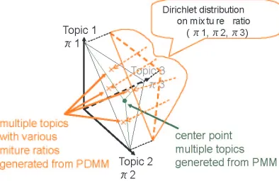
In Figure 1, the mixture ratio(bias) π = (π1, π2, π3),

P3

i=1πi = 1, πi >0of three topics is

expressed in 3-dimensional real spaceR3. The mix-ture ratio(bias)πconstructs 2D-simplex inR3. One point on the simplex indicates one mixture ratioπof the three topics. That is, the point indicates multiple topics with the mixture ratio. PMM generates doc-uments assuming that each mixture ratio is equal. That is, PMM generates only documents with mul-tiple topics that indicates the center point of the 2D-simplex in Figure 1. On the contrary, PDMM gen-erates documents assuming that mixture ratioπ fol-lows Dirichlet distribution. That is, PDMM can gen-erate documents with multiple topics whose weights can be generated by Dirichlet distribution.

4.2 Formulation

PDMM is formulated as follows: P(w|y, α, θ)

=

Z

P(π|α, y)ΠV_v=1(ϕ(v,y, θ, π))xv_{dπ (4)}

Figure 1: Topic Simplex for Three Topics

πis a vector whose element isπi(i∈Iy). πi is a

mixture ratio(bias) of model parameter correspond-ing to scorrespond-ingle topiciwhere πi > 0,P_i∈Iyπi = 1.

πican be considered as a probability of topici, i.e.,

πi = P(yi = 1|π). P(π|α, y) is a prior

distri-bution ofπ whose indexiis an element ofIy, i.e.,

i∈Iy. We use Dirichlet distribution as the prior. α

is a parameter vector of Dirichlet distribution corre-sponding toπi(i∈ Iy). Namely, the formulation is

as follows.

P(π|α, y) = Γ(

P

i∈Iyαi)

Πi∈IyΓ(αi)

Πi∈Iyπ

αi−1

i (5)

ϕ(v,y, θ, π)is the probability that wordvis gener-ated from multiple topicsyand is denoted as a linear sum ofπi(i∈Iy)andθiv(i∈Iy)as follows.

ϕ(v,y, θ, π) =X

i∈Iy

πiθiv (6)

=X

i∈Iy

P(yi= 1|π)P(v|yi= 1, θ) (7)

4.3 Variational Bayes Method for Estimating Mixture Ratio

Use Eqs.(4)(7). P(w, π|y, α, θ) =

P(π|α, y)ΠV_v=1(X

i∈Iy

P(yi = 1|π)P(v|yi = 1, θ))xv

Transform document expression of above equa-tion into words vectorw= (w1, w2,· · · , wN).

P(w, π|y, α, θ) =

P(π|α, y)ΠN_n=1 X

in∈Iy

P(yin = 1|π)P(wn|yin = 1, θ)

By changing the order of P

and Π, we have P(w, π|y, α, θ) =

P(π|α, y) X

i∈IN y

ΠN_n=1P(yin = 1|π)P(wn|yin= 1, θ)

(X

i∈IN y

≡ X

i1∈Iy

X

i2∈Iy

· · · X

iN∈Iy

)

Expressyin = 1aszn=i.

P(w|y, α, θ) =

Z X

z∈IN y

P(π|α, y)ΠN_n=1P(zn|π)P(wn|zn, θ)dπ

(X

z∈IN y

≡ X

z1∈Iy

X

z2∈Iy

· · · X

zN∈Iy

) (8)

Eq.(8) is regarded as Eq.(4) rewritten by introducing a new latent variablez= (z1, z2,· · · , zN).

P(w|y, α, θ) =

Z X

z∈IN y

P(π, z, w|y, α, θ)dπ (9)

Use Eqs.(8)(9)

P(π, z, w|y, α, θ)

=P(π|α, y)ΠN_n=1P(zn|π)P(wn|zn, θ) (10)

Hereafter, we explain Variational Bayes Method for estimating an approximate distribution of P(π, z|w, y, α, θ)using Eq.(10). This approach is the same as LDA(D.M.Blei et al., 2001; D.M.Blei et al., 2003). The approximate distribution is assumed to beQ(π, z|γ, φ). The following assumptions are introduced.

Q(π, z|γ, φ) =Q(π|γ)Q(z|φ) (11)

Q(π|γ) = Γ(

P

i∈Iyγi)

Πi∈IyΓ(γi)

Πi∈Iyπ

γi−1

i (12)

Q(z|φ) = ΠN_n=1Q(zn|φ) (13)

Q(zn|φ) = ΠKi=1(φni)z

i

n ₍₁₄₎

Q(π|γ) is Dirichlet distribution where γ is its pa-rameter.Q(zn|φ)is Multinomial distribution where

φni is its parameter and indicates the probability

that the nth word of a document is topic i, i.e. P(yin = 1). z

i

nis a value of 1(0) whenznis (not)

i. According to Eq.(11), Q(π|γ)is regarded as an approximate distribution ofP(π|w, y, α, θ)

The log likelihood ofP(w|y, α, θ)is derived as follows.

logP(w|y, α, θ)

=

Z X

z∈IN y

Q(π, z|γ, φ)dπlogP(w|y, α, θ)

=

Z X

z∈IN y

Q(π, z|γ, φ) logP(π, z, w|y, α, θ)

Q(π, z|γ, φ) dπ

+

Z X

z∈IN y

Q(π, z|γ, φ) log Q(π, z|γ, φ)

P(π, z|w, y, α, θ)dπ

logP(w|y, α, θ) =F[Q] +KL(Q, P) (15)

F[Q] =R P_z∈IN

y Q(π,z|γ,φ) log

P(π,z,w|y,α,θ)

Q(π,z|γ,φ) dπ KL(Q, P) =R P_z∈IN

y Q(π,z|γ,φ) log

Q(π,z|γ,φ)

P(π,z|w,y,α,θ)dπ KL(Q, P) is the Kullback-Leibler Divergence that is often employed as a distance between probability distributions. Namely, KL(Q, P) indicates a distance between Q(π, z|γ, φ) and P(π, z|w, y, α, θ). logP(w|y, α, θ) is not relevant toQ(π, z|γ, φ). Therefore,Q(π, z|γ, φ) that maximizes F[Q] minimizes KL(Q, P), and gives a good approximate distribution of P(π, z|w, y, α, θ).

We estimateQ(π, z|γ, φ), concretely its param-eterγandφ, by maximizingF[Q]as follows.

Using Eqs.(10)(11).

F[Q] =

Z

Q(π|γ) logP(π|α, y)dθ (16)

+

Z X

z∈IN y

Q(π|γ)Q(z|φ) log ΠN_n=1P(zn|π)dθ(17)

+ X

z∈IN y

Q(z|φ) log ΠN_n=1P(wn|zn, θ) (18)

− Z

Q(π|γ) logQ(π|γ)dθ (19)

− X

z∈IN y

= log Γ(P

i∈Iyαj)−

P

i∈Iylog Γ(αi)

+P

i∈Iy(αi−1)(Ψ(γi)−Ψ(

P

j∈Iyγj))(21)

+

N

X

n=1 X

i∈Iy

φni(Ψ(γi)−Ψ(

X

j∈Iy

γj)) (22)

+

N

X

n=1 X

i∈Iy

V

X

j=1

φniwnjlogθij (23)

− log Γ(X

j∈Iy

γj) +

X

i∈Iy

log Γ(X

j∈Iy

γj)

−X

i∈Iy

(γi−1)(Ψ(γi)−Ψ(

X

j∈Iy

γj))(24)

−

N

X

n=1 X

i∈Iy

φnilogφni (25)

F[Q]is known to be a function ofγi andφnifrom

Eqs.(21) through (25). Then we only need to re-solve the maximization problem of nonlinear func-tion F[Q]with respect toγi andφni. In this case,

the maximization problem can be resolved by La-grange multiplier method.

First, regard F[Q] as a function of γi, which

is denoted as F[γi]. Then ,γi does not have

con-straints. Therefore we only need to find the follow-ing γi, where ∂F_∂γ[γ_ii] = 0. The resultant γi is

ex-pressed as follows.

γi =αi+ N

X

n=1

φni (i∈Iy) (26)

Second, regardF[Q]as a function ofφni, which is

denoted asF[φni]. Then, considering the constraint

thatP

i∈Iyφni= 1, Lagrange functionL[φni]is

ex-pressed as follows:

L[φni] =F[φni] +λ(

X

i∈Iy

φni−1) (27)

λis a so-called Lagrange multiplier.

We find the followingφniwhere ∂L_∂φni[φni] = 0.

φni=

θiwn

C exp(Ψ(γi)−Ψ(

X

j∈Iy

γj)) (i∈Iy))(28)

Cis a normalization term. By Eqs.(26)(28), we ob-tain the following updating formulas ofγiandφni.

γ_i(t+1)=αi+ N

X

n=1

φ(_nit) (i∈Iy) (29)

φ(_nit+1) = θiwn

C exp(Ψ(γ

(t+1)

i )−Ψ(

X

j∈Iy

γ_j(t+1)))(30)

Using the above updating formulas , we can es-timate parametersγ andφ, which are specific to a documentwand topics y.Last of all , we show a pseudo code :vb(w, y)which estimatesγ andφ. In addition , we regardα , which is a parameter of a prior distribution ofπ, as a vector whose elements are all one. That is because Dirichlet distribution where each parameter is one becomes Uniform dis-tribution.

•Variational Bayes Method for PDMM———— function vb(w, y):

1. Initializeαi←1∀i∈Iy

2. Computeγ(t+1), φ(t+1)using Eq.(29)(30) 3. ifkγ(t+1)−γ(t)k<

&kφ(t+1)_−φ(t)_k<

4. then return(γ(t+1), φ(t+1))and halt 5. elset←t+ 1and goto step (2)

————————————————————

4.4 Computing Probability of Generating Document

PMM computes a probability of generating a docu-mentwon topicsyand a set of model parameterΘ as follows:

P(w|y,Θ) = ΠV_v=1(ϕ(v,y, θ))xv ₍₃₁₎

ϕ(v,y, θ) is the probability of generating a word v on topics y that is a mixture of model parame-terθiv(i ∈ Iy) with an equal mixture ratio. On the

other hand, PDMM computes the probability of gen-erating a wordvon topics yusing θiv(i ∈ Iy)and

ϕ(v,y, θ, γ)

=

Z

(X

i∈Iy

πiθiv)Q(π|γ)dπ (32)

= X

i∈Iy

Z

πiQ(π|γ)dπθiv (33)

= X

i∈Iy

˜

πiθiv (34)

˜

πi =

R

πiQ(π|γ)dπ = P γi

j∈Iyγj (C.M.Bishop,

2006)

The above equation regards the mixture ratio of topicsyof a documentwas the expectationπ˜i(i∈

Iy) of Q(π|γ). Therefore, a probability of

gener-atingwP(w|y,Θ)is computed withϕ(v,y, θ, γ) estimated in the following manner:

P(w|y,Θ) = ΠV_v=1(ϕ(v,y, θ, γ)))xv ₍₃₅₎

4.5 Algorithm for Estimating Multiple Topics of Document

PDMM estimates multiple topics y∗ maximizing a probability of generating a document w∗, i.e., Eq.(35). This is the 0-1 integer problem(i.e., NP-hard problem), so PDMM uses the same approxi-mate estimation algorithm as PMM does. But it is different from PMM’s estimation algorithm in that it estimates the mixture ratios of topicsyby Varia-tional Bayes Method as shown by vb(w,y) at step 6 in the following pseudo code of the estimation algo-rithm:

•Topics Estimation Algorithm———————– function prediction(w):

1. Initialize S ← {1,2,· · · }, yi ← 0 for

i(1,2· · · , K) 2. vmax← −∞

3. whileSis not empty do 4. foreachi∈Sdo 5. yi ←1, yj∈S\i ←0

6. Computeγby vb(w, y) 7. v(i)←P(w|y)

8. end foreach 9. i∗←argmaxv(i) 10. ifv(i∗)> vmax

11. yi∗←1, S ←S\i∗, v_max ←v(i∗)

12. else

13. returnyand halt

————————————————————

5 Evaluation

We evaluate the proposed model by using F-measure of multiple topics categorization problem.

5.1 Dataset

We use MEDLINE1as a dataset. In this experiment, we use five thousand abstracts written in English. MEDLINE has a metadata set called MeSH Term. For example, each abstract has MeSH Terms such as RNA Messenger and DNA-Binding Proteins. MeSH Terms are regarded as multiple topics of an abstract. In this regard, however, we use MeSH Terms whose frequency are medium(100-999). We did that be-cause the result of experiment can be overly affected by such high frequency terms that appear in almost every abstract and such low frequency terms that ap-pear in very few abstracts. In consequence, the num-ber of topics is 88. The size of vocabulary is 46,075. The proportion of documents with multiple topics on the whole dataset is 69.8%, i.e., that of documents with single topic is 30.2%. The average of the num-ber of topics of a document is 3.4. Using TreeTag-ger2, we lemmatize every word. We eliminate stop words such as articles and be-verbs.

5.2 Result of Experiment

We compare F-measure of PDMM with that of PMM and other models.

F-measure(F) is as follows: F = _P2P R_+R, P = |Nr∩Ne|

|Ne| , R=

|Nr∩Ne|

|Nr| .

Nr is a set of relevant topics . Neis a set of

esti-mated topics. A higher F-measure indicates a better ability to discriminate topics. In our experiment, we compute F-measure in each document and average the F-measures throughout the whole document set. We consider some models that are distinct in learning model parameterθ. PDMMlearns model parameter θ by the same learning algorithm as PMM. NBM learns model parameter θ by Naive Bayes learning algorithm. The parameters are up-dated according to the following formula: θiv =

Miv+1

C . Miv is the number of training documents

where a wordvappears in topici. Cis normaliza-tion term forPV

v=1θiv= 1.

1

http://www.nlm.nih.gov/pubs/factsheets/medline.html

2

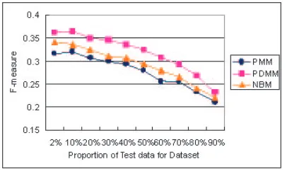
The comparison of these models with respect to F-measure is shown in Figure 2. The horizontal axis is the proportion of test data of dataset(5,000 ab-stracts). For example, 2% indicates that the number of documents for learning model is 4,900 and the number of documents for the test is 100. The vertical axis is F-measure. In each proportion, F-measure is an average value computed from five pairs of train-ing documents and test documents randomly gener-ated from dataset.

F-measure of PDMM is higher than that of other methods on any proportion, as shown in Figure 2. Therefore, PDMM is more effective than other methods on multiple topics categorization.

Figure 3 shows the comparison of models with respect to F-measure, changing proportion of mul-tiple topic document for the whole dataset. The pro-portion of document for learning and test are 40% and 60%, respectively. The horizontal axis is the proportion of multiple topic document on the whole dataset. For example, 30% indicates that the pro-portion of multiple topic document is 30% on the whole dataset and the remaining documents are sin-gle topic , that is, this dataset is almost sinsin-gle topic document. In 30%. there is little difference of F-measure among models. As the proportion of mul-tiple topic and single topic document approaches 90%, that is, multiple topic document, the differ-ences of F-measure among models become appar-ent. This result shows that PDMM is effective in modeling multiple topic document.

Figure 2: F-measure Results

5.3 Discussion

In the results of experiment described in section 5.2, PDMM is more effective than other models in

Figure 3: F-measure Results changing Proportion of Multiple Topic Document for Dataset

multiple-topic categorization. If the topic weight-ings are averaged over all biases in the whole of training documents, they could be canceled. This cancellation can lead to the result that model pa-rameter θ learned by PMM is reasonable over the whole of documents. Moreover, PDMM computes the probability of generating a document using a mixture of model parameter, estimating the mixture ratio of topics. This estimation of the mixture ra-tios, we think, is the key factor to achieve the re-sults better than other models. In addition, the es-timation of a mixture ratio of topics can be effec-tive from the perspeceffec-tive of extracting features of a document with multiple topics. A mixture ratio of topics assigned to a document is specific to the document. Therefore, the estimation of the mixture ratio of topics is regarded as a projection from a word-frequency space of QV where Q is a set of integer number to a mixture ratio space of topics [0,1]K in a document. Since the size of vocabu-lary is much more than that of topics, the estima-tion of the mixture ratio of topics is regarded as a dimension reduction and an extraction of features in a document. This can lead to analysis of similarity among documents with multiple topics. For exam-ple, the estimated mixture ratio of topics [Compara-tive Study]C[Apoptosis] and [Models,Biological] in one MEDLINE abstract is 0.656C0.176 and 0.168, respectively. This ratio can be a feature of this doc-ument.

Table 1: Word List of Document X whose Topics are [Female], [Male] and [Biological Markers]

Ranking Top10 Ranking Bottom10 1(37) biomarkers 67(69) indicate

2(19) Fusarium 68(57) problem

3(20) non-Gaussian 69(45) use 4(21) Stachybotrys 70(75) % 5(7) chrysogenum 71(59) correlate 6(22) Cladosporium 72(17) population

7(3) mould 73(15) healthy

8(35) Aspergillus 7433) response

9(23) dampness 75(56) man

10(24) 1SD 76(64) woman

φniindicates the probability that a wordwnbelongs

to topiciin a document. Therefore we can compute the entropy onwnas follows:

entropy(wn) =

PK

i=1φnilog(φni)

We rank words in a document by this entropy. For example, a list of words in ascending order of the entropy in document X is shown in Table 1. A value in parentheses is a ranking of words in decending or-der of TF-IDF(= tf ·log(M/df),wheretf is term frequency in a test document, df is document fre-quency andMis the number of documents in the set of doucuments for learning model parameters) (Y. Yang and J. Pederson, 1997) . The actually assigned topics are [Female] , [Male] and [Biological Mark-ers], where each estimated mixture ratio is 0.499 , 0.460 and 0.041, respectively.

The top 10 words seem to be more technical than the bottom 10 words in Table 1. When the entropy of a word is lower, the word is more topic-specific ori-ented, i.e., more technical . In addition, this ranking of words depends on topics assigned to a document. When we assign randomly chosen topics to the same document, generic terms might be ranked higher. For example, when we rondomly assign the topics [Rats], [Child] and [Incidence], generic terms such as ”use” and ”relate” are ranked higher as shown in Table 2. The estimated mixture ratio of [Rats], [Child] and [Incidence] is 0.411, 0.352 and 0.237, respectively.

For another example, a list of words in ascending order of the entropy in document Y is shown in Ta-ble 3. The actually assigned topics are Female, An-imals, Pregnancy and Glucose.. The estimated mix-ture ratio of [Female], [Animals] ,[Pregnancy] and

Table 2: Word List of Document X whose Topics are [Rats], [Child] and [Incidence]

Ranking Top10 Ranking Bottom10

1(69) indicate 67(56) man

2(63) relate 68(47) blot

3(53) antigen 69(6) exposure

4(45) use 70(54) distribution

5(3) mould 71(68) evaluate

6(4) versicolor 72(67) examine 7(35) Aspergillus 73(59) correlate 8(7) chrysogenum 74(58) positive

9(8) chartarum 75(1) IgG

10(9) herbarum 76(60) adult

[Glucose] is 0.442, 0.437, 0.066 and 0.055, respec-tively In this case, we consider assigning sub topics of actual topics to the same document Y.

Table 4 shows a list of words in document Y as-signed with the sub topics [Female] and [Animals]. The estimated mixture ratio of [Female] and [An-imals] is 0.495 and 0.505, respectively. Estimated mixture ratio of topics is chaged. It is interesting that [Female] has higher mixture ratio than [Ani-mals] in actual topics but [Female] has lower mix-ture ratio than [Animals] in sub topics [Female] and [Animals]. According to these different mixture ra-tios, the ranking of words in docment Y is changed.

Table 5 shows a list of words in document Y as-signed with the sub topics [Pregnancy] and [Glu-cose]. The estimated mixture ratio of [Pregnancy] and [Glucose] is 0.502 and 0.498, respectively. It is interesting that in actual topics, the ranking of gglucose-insulinh and ”IVGTT” is high in document Y but in the two subset of actual topics, gglucose-insulinh and ”IVGTT” cannot be find in Top 10 words.

Table 3: Word List of Document Y whose Ac-tual Topics are [Femaile],[Animals],[Pregnancy] and [Glucose]

Ranking Top 10 Ranking Bottom 10 1(2) glucose-insulin 94(93) assess

2(17) IVGTT 95(94) indicate

3(11) undernutrition 96(74) CT

4(12) NR 97(28) %

5(13) NRL 98(27) muscle

6(14) GLUT4 99(85) receive

7(56) pregnant 100(80) status 8(20) offspring 101(100) protein

9(31) pasture 102(41) age

10(32) singleton 103(103) conclusion

Table 4: Word List of Document Y whose Topics are [Femaile]and [Animals]

Ranking Top 10 Ranking Bottom 10

1(31) pasture 94(65) insulin

2(32) singleton 95(76) reduced

3(33) insulin-signaling 96(27) muscle

4(34) CS 97(74) CT

5(35) euthanasia 98(68) feed

6(36) humane 99(100) protein

7(37) NRE 100(80) status

8(38) 110-term 101(85) receive

9(50) insert 102(41) age

10(11) undernutrition 103(103) conclusion

6 Concluding Remarks

We proposed and evaluated a novel probabilistic generative models, PDMM, to deal with multiple-topic documents. We evaluated PDMM and other models by comparing F-measure using MEDLINE corpus. The results showed that PDMM is more ef-fective than PMM. Moreover, we indicate the poten-tial of the proposed model that extracts document-specific keywords using information of assigned topics.

Acknowledgement This research was funded in part by MEXT Grant-in-Aid for Scientific Research on Priority Areas ”i-explosion” in Japan.

References

H.Attias 1999. Learning parameters and structure of la-tent variable models by variational Bayes. in Proc of Uncertainty in Artificial Intelligence.

C.M.Bishop 2006. Pattern Recognition And Machine

Table 5: Word List of Document Y whose Topics are [Pregnancy]and [Glucose]

Ranking Top 10 Ranking Bottom 10

1(84) mass 94(18) IVGTT

2(74) CT 95(72) metabolism

3(26) requirement 96(73) metabolic 4(45) intermediary 97(57) pregnant 5(50) insert 98(58) prenatal 6(53) feeding 99(59) fetal 7(55) nutrition 100(3) gestation 8(61) nutrient 101(20) offspring 9(31) pasture 102(65) insulin 10(32) singleton 103(16) glucose

Learning (Information Science and Statistics), p.687. Springer-Verlag.

D.M. Blei, Andrew Y. Ng, and M.I. Jordan. 2001. Latent Dirichlet Allocation. Neural Information Processing Systems14.

D.M. Blei, Andrew Y. Ng, and M.I. Jordan. 2003. La-tent Dirichlet Allocation. Journal of Machine Learn-ing Research, vol.3, pp.993-1022.

Minka 2002. Estimating a Dirichlet distribution. Techni-cal Report.

Y.W.Teh, M.I.Jordan, M.J.Beal, and D.M.Blei. 2003. Hierarchical dirichlet processes. Technical Report 653, Department Of Statistics, UC Berkeley.

Ueda, N. and Saito, K. 2002. Parametric mixture models for multi-topic text. Neural Information Processing Systems15.

Ueda, N. and Saito, K. 2002. Singleshot detection of multi-category text using parametric mixture models. ACM SIG Knowledge Discovery and Data Mining.