Proceedings of the 2011 Conference on Empirical Methods in Natural Language Processing, pages 552–561, Edinburgh, Scotland, UK, July 27–31, 2011. c2011 Association for Computational Linguistics
Semantic Topic Models: Combining Word Distributional Statistics and
Dictionary Definitions
Weiwei Guo
Department of Computer Science, Columbia University, [email protected]
Mona Diab
Center for Computational Learning Systems, Columbia University,
Abstract
In this paper, we propose a novel topic model based on incorporating dictionary definitions. Traditional topic models treat words as surface strings without assuming predefined knowledge about word mean-ing. They infer topics only by observing surface word co-occurrence. However, the co-occurred words may not be semanti-cally related in a manner that is relevant for topic coherence. Exploiting dictionary definitions explicitly in our model yields a better understanding of word semantics leading to better text modeling. We exploit WordNet as a lexical resource for sense definitions. We show that explicitly mod-eling word definitions helps improve per-formance significantly over the baseline for a text categorization task.
1 Introduction
Latent Dirichlet Allocation (LDA) (Blei et al., 2003) serves as a data-driven framework in model-ing text corpora. The statistical model allows vari-able extensions to integrate linguistic features such as syntax (Griffiths et al., 2005), and has been ap-plied in many areas.
In LDA, there are two factors which determine the topic of a word: the topic distribution of the document, and the probability of a topic to emit this word. This information is learned in an unsu-pervised manner to maximize the likelihood of the corpus. However, this data-driven approach has some limitations. If a word is not observed fre-quently enough in the corpus, then it is likely to be assigned the dominant topic in this document. For example, the wordgrease (a thick fatty oil)in a political domain document should be assigned the topic chemicals. However, since it is an in-frequent word, LDA cannot learn its correct se-mantics from the observed distribution, the LDA
model will assign it the dominant document topic
politics. If we look up the semantics of the word
grease in a dictionary, we will not find any of its
meanings indicating thepoliticstopic, yet there is ample evidence for the chemicaltopic. Accord-ingly, we hypothesize that if we know the seman-tics of words in advance, we can get a better in-dication of their topics. Therefore, in this paper, we test our hypothesis by exploring the integration of word semantics explicitly in the topic modeling framework.
In order to incorporate word semantics from dictionaries, we recognize the need to model sense-topic distribution rather than word-topic dis-tribution, since dictionaries are constructed at the sense level. We use WordNet (Fellbaum, 1998) as our lexical resource of choice. The notion of a sense in WordNet goes beyond a typical word sense in a traditional dictionary since a WordNet sense links senses of different words that have similar meanings. Accordingly, the sense for the first verbal entry for buy and for purchase will have the same sense id (and same definition) in WordNet, while they could have different mean-ing definitions in a traditional dictionary such as the Merriam Webster Dictionary or LDOCE. In our model, a topic will first emit a WordNet sense, then the sense will generate a word. This is in-spired by the intuition that words are instantiations of concepts.
The paper is organized as follows: In Sections 2 and 3, we describe our models based on WordNet. In Section 4, experiment results on text catego-rization are presented. Moreover, we analyze both qualitatively and quantitatively the contribution of modeling definitions (by teasing out the contribu-tion of explicit sense modeling in a word sense dis-ambiguation task). Related work is introduced in Section 5. We conclude in Section 6 by discussing some possible future directions.
d
(a)
d
T
S
sen
sen
γ/Nsen
d s
(b)
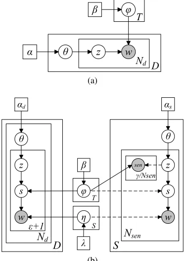
Figure 1: (a) LDA: Latent Dirichlet Allocation (Blei et al., 2003). (b) STM: Semantic topic model. The dashed arrows indicate the distribu-tions (φandη) and nodes (z) are not influenced by the values of pointed nodes.
2 Semantic Topic Model
2.1 Latent Dirichlet Allocation
We briefly introduce LDA where Collapsed Gibbs Sampling (Griffiths and Steyvers, 2004) is used for inference. In figure 1a, given a corpus with
D documents, LDA will summarize each
docu-ment as a normalizedT-dimension topic mixture
θ. Topic mixtureθis drawn from a Dirichlet
distri-butionDir(α)with a symmetric priorα. φ
con-tainsT multinomial distribution, each represent-ing the probability of a topiczgenerating wordw p(w|z). φ is drawn from a Dirichlet distribution Dir(β)with priorβ.
In Collapsed Gibbs Sampling, the distribution of a topic for the wordwi =wbased on values of
other data is computed as:
P(zi=z|z−i,w)∝
n(d)−i,z+α
n(d)−i+T α × n
w
−i,z+β
n−i,z+W β (1)
In this equation,n(−di,z) is a count of how many
words are assigned topiczin documentd,
exclud-ing the topic of theith word; nw
−i,z is a count of
how many words= w are assigned topicz, also
excluding the topic of the ith word. Hence, the
first fraction is the proportion of the topic in this documentp(z|θ). The second fraction is the
prob-ability of topiczemitting wordw. After the topics
become stable, all the topics in a document con-struct the topic mixtureθ.
2.2 Applying Word Sense Disambiguation Techniques
We add a sense node between the topic node and the word node based on two linguistic observa-tions: a) Polysemy: many words have more than one meaning. A topic is more directly relevant to a word meaning (sense) than to a word due to pol-ysemy; b)Synonymy: different words may share the same sense. WordNet explicitly models syn-onymy by linking synonyms to the same sense. In WordNet, each sense has an associated definition. It is worth noting that we model the sense-word relation differently from (Boyd-Graber and Blei, 2007), where in their model words are generated from topics, then senses are generated from words. In our model, we assume that during the genera-tive process, the author picks a concept relevant to the topic, then thinks of a best word that represents that concept. Hence the word choice is dependent on the relatedness of the sense and its fit to the document context.
In standard topic models, the topic of a word is sampled from the document level topic mixture
θ. The underlying assumption is that all words in a
document constitute the context of the target word. However, it is not the case in real world corpora. Titov and McDonald (2008) find that using global topic mixtures can only extract global topics in on-line reviews (e.g., Creative Labs MP3 players and iPods) and ignores local topics (product features such as portability and battery). They design the Multi-grain LDA where the local topic of a word is only determined by topics of surrounding sen-tences. In word sense disambiguation (WSD), an even narrower context is taken into consideration, for instance in graph based WSD models (Mihal-cea, 2005), the choice of a sense for a word only depends on a local window whose size equals the length of the sentence. Later in (Sinha and Mihal-cea, 2007; Guo and Diab, 2010; Li et al., 2010), people use a fixed window size containing around 12 neighbor words for WSD.
[image:2.612.96.285.39.302.2]not employ the complicated schema in (Titov and McDonald, 2008). We simply hypothesize that the surroundingwords are semantically related to the
considered word, and they construct a local slid-ing window for that target word. For a document
dwithNdwords, we represent it asNdlocal
win-dows – a window is created for each word. The model is illustrated in the left rectangle in figure 1b. The window size is fixed for each word: it contains/2 preceding words, and/2 following
words. Therefore, a word in the original document will havecopies, existing in+ 1local windows.
Similarly, there are + 1 pairs of topics/senses
assigned for each word in the original document. Each window has a distributionθiover topics. θi
will emit the topics of words in the window. This approach enables us to exploit different context sizes without restricting it to the sentence length, and hence spread topic information across sentence boundaries.
2.3 Integrating Definitions
Intuitively, a sense definition reveals some prior knowledge on the topic domain: the definition of sense [crime, offense, offence] indicates a legal
topic; the definition of sense [basketball] indicates
asportstopic, etc. Therefore, during inference, we
want to choose a topic/sense pair for each word, such that the topic is supported by the context θ
and the sense definition also matches that topic. Given that words used in the sense definitions are strongly relevant to the sense/concept, we set out to find the topics of those definition words, and accordingly assign the sensesenitself these
top-ics. We treat a sense definition as a document and perform Gibbs sampling on it. We normalize def-inition length by a variableγ. Therefore, before
the topic model sees the actual documents, each sense shas been sampled γ times. Theγ topics
are then used as a “training set”, so that given a sense,φhas some prior knowledge of which topic
it should be sampled from.
Consider the sense [party, political party] with a definition “an organization to gain political
power” of length 6 when γ = 12. If topic
model assignspolitics topic to the words “orga-nization political power”, then sense [party,
polit-ical party] will be sampled frompoliticstopic for
3∗γ/def initionLength= 6times.
We refer to the proposed model as Semantic Topic Model (figure 1b). For each windowvi in
the document set, the model will generate a distri-bution of topicsθi. It will emit the topics of+ 1
words in the window. For a wordwij in window vi, a sensesij is drawn from the topic, and thensij
generates the wordwi. Sense-topic distributionφ
containsT multinomial distributions over all
pos-sible senses in the corpus drawn from a symmetric Dirichlet distributionDir(β). From WordNet we
know the set of words W(s) that have a senses
as an entry. A sense scan only emit words from W(s). Hence, for each senses, there is a
multi-nomial distributionηsoverW(s). Allηare drawn
from symmetricDir(λ).
On the definition side, we use a different prior
αsto generate a topic mixtureθ. Aside from
gen-erating si, zi will deterministically generate the
current sense sen for γ/Nsen times (Nsen is the
number of words in the definition of sense sen),
so thatsenis sampledγtimes in total.
The formal procedure of generative process is the following:
For the definition of sensesen:
•choose topic mixtureθ∼Dir(αs).
•for each wordwi:
−choose topiczi ∼M ult(θ).
−choose sensesi∼M ult(φzi).
− deterministically choose sense sen ∼
M ult(φzi)forγ/Nsentimes. −choose wordwi∼M ult(ηsi).
For each windowvi in a document:
•choose local topic mixtureθi ∼Dir(αd).
•for each wordwij invi:
−choose topiczij ∼M ult(θi).
−choose sensesij ∼M ult(φzij). −choose wordwij ∼M ult(ηsij).
2.4 Using WordNet
Since definitions and documents are in different genre/domains, they have different distributions on senses and words. Besides, the definition sets contain topics from all kinds of domains, many of which are irrelevant to the document set. Hence we prefer φ and η that are specific for the
doc-ument set, and we do not want them to be “cor-rupted” by the text in the definition set. There-fore, as in figure 1b, the dashed lines indicate that when we estimateφandη, the topic/sense pair and sense/word pairs in the definition set are not con-sidered.
We observe that neighboring sense definitions are usually similar and are in the same topic domain. Hence, we represent the definition of a sense as the union of itself with its neighboring sense def-initions pertaining to WordNet relations. In this way, the definition gets richer as it considers more data for discovering reliable topics.
3 Inference
We still use Collapsed Gibbs Sampling to find la-tent variables. Gibbs Sampling will initialize all hidden variables randomly. In each iteration, hid-den variables are sequentially sampled from the distribution conditioned on all the other variables. In order to compute the conditional probability
P(zi = z, si = s|z−i,s−i,w) for a topic/sense pair, we start by computing the joint probability
P(z,s,w) =P(z)P(s|z)P(w|s). Since the
gen-erative processes are not exactly the same for def-initions and documents, we need to compute the joint probability differently. We use a type spe-cific subscript to distinguish them:Ps(·)for sense
definitions andPd(·)for documents.
Letsenbe a sense. Integrating outθwe have:
Ps(z) =
Γ(T αs)
Γ(αs)T S YS
sen=1 Q
zΓ(n (sen) z +αs)
Γ(n(sen)+T α) (2)
wheren(zsen) means the number of times a word
in the definition ofsenis assigned to topicz, and n(sen) is the length of the definition. S is all the potential senses in the documents.
We have the same formula of P(s|z) and
P(w|s)for definitions and documents. Similarly,
let nz be the number of words in the documents
assigned to topicz, andns
zbe the number of times
sense s assigned to topic z. Note that when s
appears in the superscript surrounded by brackets such as n(zs), it denotes the number of words
as-signed to topicszin the definition of senses. By
integrating outφwe obtain the second term:
P(s|z) =
Γ(Sβ)
Γ(β)S TYT
z=1 Q
sΓ(n s
z+n(s)z γ/n(s)+β)
Γ(nz+Ps0n(s 0)
z γ/n(s0)+Sβ) (3)
At last, assumensdenotes the number of sense sin the documents, andnws denotes the number of
sense sto generate the word w, then integrating
outηwe have:
P(w|s) =
S Y
s=1
Γ(|W(s)|λ) Γ(λ)|W(s)|
QW(s) w Γ(n
w s +λ)
Γ(ns+|W(s)|λ) (4)
With equation 2-4, we can compute the condi-tional probability Ps(zi = z, si = s|z−i,s−i,w) for a sense-topic pair in the sense definition. Let
seni be the sense definition containing word wi,
then we have:
Ps(zi=z, si=s|z−i,s−i,w)∝
n(seni)
−i,z +αs
n(seni)
−i +T αs
ns z+n
(s0)
−i,zγ/n(s
0)
+β
nz+Ps0n(s 0)
−i,zγ/n(s0)+Sβ
nw s +λ
ns+|W(s)|λ
(5)
The subscript −i in expression n−i denotes
the number of certain events excluding word wi.
Hence the three fractions in equation 5 correspond to the probability of choosingzfromθsen,
choos-ingsfromzand choosingwfroms. Also note that
our model definessthat can only generate words
in W(s), therefore for any wordw /∈ W(s), the third fraction will yield a0.
The probability for documents is similar to that for definitions except that there is a topic mixture for each word, which is estimated by the topics in the window. HencePd(z)is estimated as:
Pd(z) = Y
i
Γ(T αd)
Γ(αd)T Q
zΓ(n (vi) z +αd)
Γ(n(vi)+T αd) (6) Thus, the conditional probability for documents can be estimated by cancellation terms in equation 6, 3, and 4:
Pd(zij=z, sij=s|z−ij,s−ij,w)∝
n(vi)
−ij,z+αd
n(vi)
−ij+T αd
ns
−ij,z+n (s0) z γ/n(s
0)
+β
n−ij,z+Ps0n
(s0)
z γ/n(s0)+Sβ
nw
−ij,s+λ
n−ij,s+|W(s)|λ (7)
3.1 Approximation
In current model, each word appears in+ 1
win-dows, and will be generated+ 1times, so there
will be + 1 pairs of topics/senses sampled for
each word, which requires a lot of additional com-putation (proportional to context size ). On the
other hand, it can be imagined that the set of val-ues {zij, sij|j − /2 ≤ i ≤ j + /2} in
dif-ferent windows vi should roughly be the same,
since they are hidden values for the same wordwj.
Therefore, to reduce computation complexity dur-ing Gibbs sampldur-ing, we approximate the values of
{zij, sij|i =6 j}by the topic/sense (zjj, sjj) that
are generated from window vj. That is, in Gibbs
sampling, the algorithm does not actually sample the values of{zij, sij,|i6=j}; instead, it directly
assumes the sampled values arezjj, sjj.
4 Experiments and Analysis
Data: We experiment with several datasets, namely, the Brown Corpus (Brown), New York Times (NYT) from the American National Cor-pus, Reuters (R20) and WordNet definitions. In a preprocessing step, we remove all the non-content words whose part of speech tags are not one of the following set{noun, adjective, adverb, verb}. Moreover, words that do not have a valid lemma in WordNet are removed. For WordNet definitions, we remove stop words hence focusing on relevant content words.
Corpora statistics after each step of preprocess-ing is presented in Table 1. The columnWN token
lists the number of word#pos tokens after prepro-cessing. Note that now we treat word#pos as a
word token. The columnword types shows
cor-responding word#pos types, and the total number of possible sense types is listed in column sense
types. The DOCs size for WordNet is the total
number of senses defined in WordNet.
Experiments: We design two tasks to test our models: (1) text categorization task for evaluat-ing the quality of values of topic nodes, and (2) a WSD task for evaluating the quality of the values of the sense nodes, mainly as a diagnostic tool tar-geting the specific aspect of sense definitions in-corporation and distinguish that component’s con-tribution to text categorization performance. We compare the performance of four topic models. (a) LDA: the traditional topic model proposed in (Blei et al., 2003) except that it uses Gibbs Sam-pling for inference. (b) LDA+def: is LDA with sense definitions. However they are not explic-itly modeled; rather they are treated as documents and used as augmented data. (c) STM0: the topic model with an additional explicit sense node in the model, but we do not model the sense definitions. And finally (d) STMn is the full model with defi-nitions explicitly modeled. In this settingnis the γ value. We experiment with different γ values in the STM models, and investigate the semantic scope of words/senses by choosing different win-dow size. We report mean and standard deviation based on 10 runs.
It is worth noting that a larger window size
suggests documents have larger impact on the
model (φ, η) than definitions, since each document
word hascopies. This is not a desirable property when we want to investigate the weight of
defi-nitions by choosing different γ values.
Accord-ingly, we only usezjj, sjj, wjjto estimateφ, η, so
that the impact of documents is fixed. This makes more sense, in that after the approximation in sec-tion 3.1, there is no need to use{zij, sij,|i 6=j}
(they have the same values aszjj, sjj).
4.1 Text Categorization
We believe our model can generate more “correct” topics by looking into dictionaries. In topic mod-els, each word is generalized as a topic and each document is summarized as the topic mixture θ,
hence it is natural to evaluate the quality of in-ferred topics in a text categorization task. We fol-low the classification framework in (Griffiths et al., 2005): first run topic models on each dataset
individually without knowing label information to achieve document level topic mixtures, then we employ Naive Bayes and SVM (both implemented in the WEKA Toolkit (Hall et al., 2009)) to per-form classification on the topic mixtures. For all document, the features are the percentage of top-ics. Similar to (Griffiths et al., 2005), we assess in-ferred topics by the classification accuracy of 10-fold cross validation on each dataset.
We evaluate our models on three datasets in the cross validation manner: The Brown corpus which comprises 500 documents grouped into 15 cate-gories (same set used in (Griffiths et al., 2005)); NYT comprising 800 documents grouped into the 16 most frequent label categories; Reuters (R20) comprising 8600 documents labeled with the most frequent 20 categories. In R20, combination of categories is treated as separate category labels, somoney, interestandinterest are considered
different labels.
For the three datasets, we use the Brown cor-pus only as a tuning set to decide on the topic model parameters for all of our experimentation, and use the optimized parameters directly on NYT and R20 without further optimization.
4.1.1 Classification Results
Searchingγ andon Brown: The classification
accuracy on the Brown corpus with differentand
γ values using Naive Bayes and SVM are
pre-sented in figure 2a and 2b. In this section, the
number of topics T is set to 50. The possible
values in the horizontal axis are 2, 10, 20, 40,
all. The possibleγ values are0, 1, 2. Note that = allmeans that no local window is used, and
γ = 0means definitions are not used. The
Corpus DOCs size orig tokens content tokens WN tokens word types sense types
Brown 500 1022393 580882 547887 27438 46645
NYT 800 743665 436988 393120 19025 37631
R20 8595 901691 450935 417331 9930 24834
SemCor 352 676546 404460 352563 28925 45973
[image:6.612.121.495.36.102.2]WordNet 117659 1447779 886923 786679 42080 60567
Table 1: Corpus statistics
0 10 20 30 40 50 all
40 45 50 55 60 65 70
window size
accuracy%
LDA LDA+def STM0 STM1 STM2
(a) Naive Bayes on Brown
0 10 20 30 40 50 all
40 45 50 55 60 65 70 75
window size
accuracy%
LDA LDA+def STM0 STM1 STM2
(b) SVM on Brown
0 10 20 30 40 50 all
55 60 65 70 75 80
window size
accuracy%
STM0 STM1 STM2
[image:6.612.98.512.147.265.2](c) SVM on NYT
Figure 2: Classification accuracy at different parameter settings
parameters are tuned asαd= 0.1, αs= 0.01, β=
0.01, λ= 0.1.
From figure 2, we observe that results using SVM have the same trend as Naive Bayes except that the accuracies are roughly 5% higher for SVM classifier. The results of LDA and LDA+def sug-gest that simply treating definitions as documents in an augmented data manner does not help.
Com-paring SMT0 with LDA in the samevalues, we
find that explicitly modeling the sense node in the model greatly improves the classification results. The reason may be that words in LDA are inde-pendent isolated strings, while in STM0 they are connected by senses.
STM2 prefers smaller window sizes (less than 40). That means two words with a distance larger than 40 are not necessarily semantically related or share the same topic. This number also corre-lates with the optimal context window size of 12 reported in WSD tasks (Sinha and Mihalcea, 2007; Guo and Diab, 2010).
Classification results: Table 2 shows the results of our models using best tuned parameters of= 10, γ = 2on 3 datasets. We present three base-lines in Table 2: (1) WEKA uses WEKA’s classi-fiers directly on bag-of-words without topic mod-eling. The values of features are simply term fre-quency. (2) WEKA+FS performs feature selection using information gain before applying classifica-tion. (3) LDA, is the traditional topic model. Note that Griffiths et al.’s (2005) implementation of
LDA achieve 51% on Brown corpus using Naive Bayes . Finally the Table illustrates the results obtained using our proposed models STM0 (γ=0) and STM2 (γ= 2).
It is worth noting that R20 (compared to NYT) is a harder condition for topic models. This is because fewer words (10000 distinct words ver-sus 19000 in NYT) are frequently used in a large training set (8600 documents versus 800 in NYT), making the surface word feature space no longer as sparse as in the NYT or Brown corpus, which implies simply using surface words without con-sidering the words distributional statistics – topic modeling – is good enough for classification. In (Blei et al., 2003) figure 10b they also show worse text categorization results over the SVM baseline when more than 15% of the training labels of Reuters are available for the SVM classifiers, indi-cating that LDA is less necessary with large train-ing data. In our investigation, we report results on SVM classifiers trained on the whole Reuters training set. In our experiments, LDA fails to cor-rectly classify nearly 10% of the Reuters docu-ments compared to the WEKA baseline, however STM2 can still achieve significantly better accu-racy (+4%) in the SVM classification condition.
Brown NYT R20
NB SVM NB SVM NB SVM
WEKA 48 47.8 57 54.1 72.4 82.9
WEKA+FS 50 47.2 56.9 55.1 72.9 83.4
[image:7.612.136.480.38.110.2]LDA 47.8±4.3 53.9±3.8 48.5±5.5 53.8±3.5 61.0±3.3 72.5±2.5 STM0 68.6±3.5 70.7±3.9 66.7±3.8 74.2±4.0 72.7±3.5 85.2±0.9 STM2 69.3±3.3 75.4±3.7 74.6±3.3 79.3±2.5 73±3.7 86.9±1.2
Table 2: Classification results on 3 datasets using hyperparameters tuned on Brown.
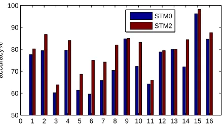
0 1 2 3 4 5 6 7 8 9 10 11 12 13 14 15 16 50
60 70 80 90 100
accuracy%
STM0 STM2
1.Sports 2.Politics 3.National News 4.Entertainment 5.International News 6.Society 7.Business 8.Miscellaneous 9.Finance 10.Culture 11.Science 12.Health 13.Law 14.Technology 15.Religion 16.Environment
Figure 3: SVM accuracy on each category of NYT
significantly better results than all three baselines including LDA. Furthermore, explicit definition modeling as used in STM2 yields the best perfor-mance consistently overall.
Finally, in Figure 2c we show the SVM clas-sification results on NYT in different parame-ter settings. We find that the NYT classifica-tion accuracy trend is consistent with that on the
Brown corpus for each parameter setting of ∈
{2,10,20,40, all}andγ ∈ {0,1,2}. This further proves the robustness of STMn.
4.2 Analysis on the Impact of Modeling Definitions
4.2.1 Qualitative Analysis
To understand why definitions are helpful in text categorization, we analyze the SVM performance
of STM0 and STM2 ( = 10) on each
cate-gory of NYT dataset (figure 3). We find STM2 outperforms STM0 in all categories. However, the largest gain is observed in Society,
Miscel-laneous, Culture, Technology. For Technology,
we should credit WordNet definitions, since
Tech-nology may contain many infrequent technical
terms, and STM0 cannot generalize the meaning of words only by distributional information due to their low frequency usage. However in some other domains, fewer specialized words are repeatedly
used, hence STM0 can do as well as STM2. For the other 3 categories, we hypothesize that these documents are likely to be a mixture of mul-tiple topics. For example, a Culture news could contain topics pertaining to religion, history, art; while a Society news about crime could relate to
law, family, economics. In this case, it is very
important to sample a true topic for each word, so that ML algorithms can distinguish the Cul-turedocuments from theReligionones by the pro-portion of topics. Accordingly, adding definitions should be very helpful, since it specifically defines the topic of a sense, and shields it from the influ-ence of other “incorrect/irrelevant” topics.
4.2.2 Quantitative Analysis with Word Sense Disambiguation
A side effect of our model is that it sense disam-biguates all words. As a means of analyzing and gaining some insight into the exact contribution of explicitly incorporating sense definitions (STMn) versus simply a sense node (STM0) in the model, we investigate the quality of the sense assignments in our models. We believe that the choice of the correct sense is directly correlated with the choice of a correct topic in our framework. Accord-ingly, a relative improvement of STMn over STM0 (where the only difference is the explicit sense def-inition modeling) in WSD task is an indicator of the impact of using sense definitions in the text categorization task.
[image:7.612.84.304.160.282.2]Total Noun Adjective Adverb Verb sense annotated words 225992 86996 31729 18947 88320
polysemous words 187871 70529 21989 11498 83855
TF-IDF - 0.422 0.300 0.153 0.182
Table 3: Statistics of SemCor per POS
statistics of SemCor is listed in table 3.
We use hyperparameters tuned from the text cat-egorization task: αd=0.1, αs=0.01, β=0.01, δ=1, T=50, and try different values of∈ {10,20,40}
andγ ∈ {0,2,10}. The Brown corpus and
Word-Net definitions corpus are used as augmented data, which means the dashed line in figure 1c will be-come bold. Finally, we choose the most frequent answer for each word in the last 10 iterations of a Gibbs Sampling run as the final sense choice.
WSD Results: Disambiguation per POS results are presented in table 4. We only report results on polysemous words. We can see that modeling definitions (STM2 and STM10) improves perfor-mance significantly over STM0’s across the board per POS and overall. The fact that STMn picks more correct senses helps explain why STMn clas-sifies more documents correctly than STM0. Also it is interesting to see that unlike in the text cate-gorization task, larger values ofγ generate better
WSD results. However, the window size, does
not make a significant difference, yet we note that
=10 is still the optimal value, similar to our
ob-servation in the text categorization task.
STM10 achieves similar results as in LDAWN (Boyd-Graber et al., 2007) which was specifically designed for WSD. LDAWN needs a fine grained hypernym hierarchy to perform WSD, hence they can only disambiguate nouns. They report differ-ent performances under various parameter setting. We cite their best performance of 38% accuracy on nouns as a comparison point to our best perfor-mance for nouns of 38.5%.
An interesting feature of STM10 is that it performs much better in nouns than adverbs and verbs, compared to a random baseline in Table 4. This is understandable since topic information content is mostly borne by nouns and adjectives, while adverbs and verbs tend to be less informa-tive about topics (e.g., even, indicate, take), and used more across different domain documents. Hence topic models are weaker in their ability to identify clear cues for senses for verbs and adverbs. In support of our hypothesis about the POS distribution, we compute the average TF-IDF
scores for each POS (shown in Table 3 according to the equation illustrated below). The average TF-IDF clearly indicate the positive skewness of the nouns and adjectives (high TF-IDF) correlates with the better WSD performance.
TF-IDF(pos) =
P i
P
dTF-IDF(wi,d)
#of wi,d where wi,d∈pos.
At last, we notice that the most frequent sense baseline performs much better than our models. This is understandable since: (1) most frequent sense baseline can be treated as a supervised method in the sense that the sense frequency is calculated based on the sense choice as present in sense annotated data; (2) our model is not de-signed for WSD, therefore it discards a lot of in-formation when choosing the sense: in our model, the choice of a sensesi is only dependent on two
facts: the corresponding topic zi and word wi,
while in (Li et al., 2010; Banerjee and Pedersen, 2003), they consider all the senses and words in the context words.
5 Related work
Various topic models have been developed for
many applications. Recently there is a trend
of modeling document dependency (Dietz et al., 2007; Mei et al., 2008; Daume, 2009). How-ever, topics are only inferred based on word co-occurrence, while word semantics are ignored.
Boyd-Graber et al. (2007) are the first to inte-grate semantics into the topic model framework. They propose a topic model based on WordNet noun hierarchy for WSD. A word is assumed to be generated by first sampling a topic, then choosing a path from the root node of hierarchy to a sense node corresponding to that word. However, they only focus on WSD. They do not exploit word def-initions, neither do they report results on text cat-egorization.
Total Noun Adjective Adverb Verb
random 22.1 26.2 27.9 32.2 15.8
most frequent sense 64.7 74.7 77.5 74.0 59.6 STM0 = 10 24.1±1.4 29.3±4.3 28.7±1.1 34.1±3.1 17.1±1.6
= 20 24±1.3 30.2±3.3 29.1±1.4 34.9±3.1 15.9±0.7
= 40 24±2.4 28.4±4.3 28.7±1.1 36.4±4.7 17.3±2.4
STM2 = 10 27.5±1.1 36.1±3.8 34.0±1.2 33.4±1.8 17.8±1.4
= 20 25.7±1.3 32.0±4.2 33.5±0.7 34.2±3.4 17.3±0.7
= 40 26.1±1.3 32.5±3.9 33.6±0.9 34.2±3.4 17.5±1.4 STM10 = 10 28.8±1.1 38.5±2.3 34.7±0.8 34.0±3.3 18.4±1.2
= 20 27.7±1.0 36.8±2.2 34.5±0.7 33.0±3.1 17.6±0.7
[image:9.612.150.466.38.161.2]= 40 28.1±1.5 38.4±3.1 34.0±1.0 35.1±5.4 17.0±0.9
Table 4: Disambiguation results per POS on polysemous words.
generated by choosing a sense path in the hierar-chy. Note that no topic information is on the sense path. If a word is generated from the hierarchy, then it is not assigned a topic. Their models based on different dictionaries improve perplexity.
Recently, several systems have been proposed to apply topic models to WSD. Cai et al. (2007) incorporate topic features into a supervised WSD framework. Brody and Lapata (2009) place the sense induction in a Baysian framework by assum-ing each context word is generated from the target word’s senses, and a context is modeled as a multi-nomial distribution over the target word’s senses rather than topics. Li et al. (2010) design sev-eral systems that use latent topics to find a most likely sense based on the sense paraphrases (ex-tracted from WordNet) and context. Their WSD models are unsupervised and outperform state-of-art systems.
Our model borrows the local window idea from word sense disambiguation community. In graph-based WSD systems (Mihalcea, 2005; Sinha and Mihalcea, 2007; Guo and Diab, 2010), a node is created for each sense. Two nodes will be con-nected if their distance is less than a predefined value; the weight on the edge is a value returned by sense similarity measures, then the PageR-ank/Indegree algorithm is applied on this graph to determine the appropriate senses.
6 Conclusion and Future Work
We presented a novel model STM that combines explicit semantic information and word distribu-tion informadistribu-tion in a unified topic model. STM is able to capture topics of words more accurately than traditional LDA topic models. In future work, we plan to model the WordNet sense network. We believe that WordNet senses are too fine-grained, hence we plan to use clustered senses, instead of
current WN senses, in order to avail the model of more generalization power.
Acknowledgments
This research was funded by the Ofce of the Direc-tor of National Intelligence (ODNI), Intelligence Advanced Research Projects Activity (IARPA), through the U.S. Army Research Lab. All state-ments of fact, opinion or conclusions contained herein are those of the authors and should not be construed as representing the ofcial views or poli-cies of IARPA, the ODNI or the U.S. Government.
References
Satanjeev Banerjee and Ted Pedersen. 2003. Extended gloss overlaps as a measure of semantic relatedness. InProceedings of the 18th International Joint Con-ference on Artificial Intelligence, pages 805–810. David M. Blei, Andrew Y. Ng, and Michael I. Jordan.
2003. Latent dirichlet allocation. Journal of
Ma-chine Learning Research, 3:993–1022.
Jordan Boyd-Graber and David M. Blei. 2007. Putop: turning predominant senses into a topic model for word sense disambiguation. InProceedings of the 4th International Workshop on Semantic Evalua-tions, pages 277–281.
Jordan Boyd-Graber, David M. Blei, and Xiaojin Zhu. 2007. A topic model for word sense disambiguation.
In Proceedings of the 2007 Joint Conference on
Empirical Methods in Natural Language Process-ing and Computational Natural Language LearnProcess-ing
(EMNLP-CoNLL), pages 1024–1033.
Samuel Brody and Mirella Lapata. 2009. Bayesian word sense induction. In Proceedings of the 12th
Conference of the European Chapter of the ACL,
pages 103–111.
Processing and Computational Natural Language
Learning, pages 1015–1023.
Chaitanya Chemudugunta, Padhraic Smyth, and Mark Steyvers. 2008. Combining concept hierarchies and statistical topic models. InProceedings of the 17th ACM conference on Information and
knowl-edge management, pages 1469–1470.
Hal Daume. 2009. Markov random topic fields. In
Proceedings of the ACL-IJCNLP Conference, pages
293–296.
Laura Dietz, Steffen Bickel, and Tobias Scheffer. 2007. Unsupervised prediction of citation influence. In Proceedings of the 24th international conference on
Machine learning, pages 233–240.
Christiane Fellbaum. 1998. WordNet: An Electronic
Lexical Database. MIT Press.
Thomas L. Griffiths and Mark Steyvers. 2004. Find-ing scientific topics. Proceedings of the National
Academy of Sciences, 101:5228–5235.
Thomas L. Griffiths, Mark Steyvers, David M. Blei, and Joshua B. Tenenbaum. 2005. Integrating top-ics and syntax. InAdvances in Neural Information Processing Systems.
Weiwei Guo and Mona Diab. 2010. Combining or-thogonal monolingual and multilingual sources of evidence for all words wsd. InProceedings of the 48th Annual Meeting of the Association for Compu-tational Linguistics, pages 1542–1551.
Mark Hall, Eibe Frank, Geoffrey Holmes, Bernhard Pfahringer, Peter Reutemann, and Ian H. Witten. 2009. The weka data mining software: an update.
SIGKDD Explor. Newsl., 11:10–18.
Linlin Li, Benjamin Roth, and Caroline Sporleder. 2010. Topic models for word sense disambiguation and token-based idiom detection. InProceedings of the 48th Annual Meeting of the Association for Com-putational Linguistics, pages 1138–1147.
Qiaozhu Mei, Deng Cai, Duo Zhang, and Chengxiang Zhai. 2008. Topic modeling with network regu-larization. InProceedings of the 17th international
conference on World Wide Web, pages 101–110.
Rada Mihalcea. 2005. Unsupervised large-vocabulary word sense disambiguation with graph-based algo-rithms for sequence data labeling. InProceedings of the Joint Conference on Human Language Tech-nology and Empirical Methods in Natural Language Processing, pages 411–418.
Sameer S. Pradhan, Edward Loper, Dmitriy Dligach, and Martha Palmer. 2007. Semeval-2007 task 17: English lexical sample, srl and all words. In Pro-ceedings of the 4th International Workshop on
Se-mantic Evaluations, pages 87–92. ACL.
Ravi Sinha and Rada Mihalcea. 2007. Unsupervised graph-based word sense disambiguation using mea-sures of word semantic similarity. InProceedings of the IEEE International Conference on Semantic
Computing, pages 363–369.
Benjamin Snyder and Martha Palmer. 2004. The en-glish all-words task. InSenseval-3: Third Interna-tional Workshop on the Evaluation of Systems for the Semantic Analysis of Text, pages 41–43. ACL.
Ivan Titov and Ryan McDonald. 2008. Modeling online reviews with multi-grain topic models. In Proceedings of the 17th international conference on
World Wide Web, pages 111–120.