Aligning context based statistical models of language with brain activity during reading

Aligning context-based statistical models of language

with brain activity during reading

Leila Wehbe1,2_{, Ashish Vaswani}3_{, Kevin Knight}3_{and Tom Mitchell}1,2

1_{Machine Learning Department, Carnegie Mellon University, Pittsburgh, PA}

2 _{Center for the Neural Basis of Computation, Carnegie Mellon University, Pittsburgh, PA}

3_{Information Sciences Institute, University of Southern California, Los Angeles, CA}

[email protected], [email protected], [email protected], [email protected]

Abstract

Many statistical models for natural language pro-cessing exist, including context-based neural net-works that (1) model the previously seen context as a latent feature vector, (2) integrate successive words into the context using some learned represen-tation (embedding), and (3) compute output proba-bilities for incoming words given the context. On the other hand, brain imaging studies have sug-gested that during reading, the brain (a) continu-ously builds a context from the successive words and every time it encounters a word it (b) fetches its properties from memory and (c) integrates it with the previous context with a degree of effort that is inversely proportional to how probable the word is. This hints to a parallelism between the neural net-works and the brain in modeling context (1 and a), representing the incoming words (2 and b) and in-tegrating it (3 and c). We explore this parallelism to better understand the brain processes and the neu-ral networks representations. We study the align-ment between the latent vectors used by neural net-works and brain activity observed via Magnetoen-cephalography (MEG) when subjects read a story. For that purpose we apply the neural network to the same text the subjects are reading, and explore the ability of these three vector representations to pre-dict the observed word-by-word brain activity. Our novel results show that: before a new wordi

is read, brain activity is well predicted by the neural network latent representation of context and the pre-dictability decreases as the brain integrates the word and changes its own representation of context. Sec-ondly, the neural network embedding of wordican predict the MEG activity when wordiis presented to the subject, revealing that it is correlated with the brain’s own representation of wordi. Moreover, we obtain that the activity is predicted in different re-gions of the brain with varying delay. The delay is consistent with the placement of each region on the processing pathway that starts in the visual cortex and moves to higher level regions. Finally, we show that the output probability computed by the neural networks agrees with the brain’s own assessment of the probability of wordi, as it can be used to predict the brain activity after the wordi’s properties have been fetched from memory and the brain is in the process of integrating it into the context.

1 Introduction

Natural language processing has recently seen a surge in increasingly complex models that achieve

impressive goals. Models like deep neural net-works and vector space models have become pop-ular to solve diverse tasks like sentiment analy-sis and machine translation. Because of the com-plexity of these models, it is not always clear how to assess and compare their performances as they might be useful for one task and not the other. It is also not easy to interpret their very high-dimensional and mostly unsupervised representa-tions. The brain is another computational system that processes language. Since we can record brain activity using neuroimaging, we propose a new di-rection that promises to improve our understand-ing of both how the brain is processunderstand-ing language and of what the neural networks are modeling by aligning the brain data with the neural networks representations.

In this paper we study the representations of two kinds of neural networks that are built to predict the incoming word: recurrent and finite context models. The first model is the Recurrent Neural Network Language Model (Mikolov et al., 2011) which uses the entire history of words to model context. The second is the Neural Probabilistic Language Model (NPLM) which uses limited con-text constrained to the recent words (3 grams or 5 grams). We trained these models on a large Harry Potter fan fiction corpus and we then used them to predict the words of chapter 9 ofHarry Potter and the Sorcerer’s Stone (Rowling, 2012). In paral-lel, we ran an MEG experiment in which 3 subject read the words of chapter 9 one by one while their brain activity was recorded. We then looked for the alignment between the word-by-word vectors produced by the neural networks and the word-by-word neural activity recorded by MEG.

Our neural networks have 3 key constituents: a hidden layer that summarizes the history of the previous words ; an embeddings vector that sum-marizes the (constant) properties of a given word and finally the output probability of a word given

Reading comprehension is reflected in the subsequent acti-vation of the left superior temporal cortex at 200–600 ms (Halgren et al., 2002; Helenius et al., 1998; Pylkka¨nen et al., 2002, 2006; Pylkka¨nen and Marantz, 2003; Simos et al., 1997). This sustained activation differentiates between words and nonwords (Salmelin et al., 1996; Wil-son et al., 2005; Wydell et al., 2003). Apart from lexical-se-mantic aspects it also seems to be sensitive to phonological manipulation (Wydell et al., 2003).

As discussed above, in speech perception activation is concentrated to a rather small area in the brain and we have to rely on time information to dissociate between dif-ferent processes. Here, the different processes are separable both in timing and location. Because of that, one might think that it is easier to characterize language-related pro-cesses in the visual than auditory modality. However, here the difficulties appear at another level. In reading, activa-tion is detected bilaterally in the occipital cortex, along the temporal lobes, in the parietal cortex and, in vocalized reading, also in the frontal lobes, at various times with respect to stimulus onset. Interindividual variability further complicates the picture, resulting in practically excessive amounts of temporal and spatial information. The areas and time windows depicted inFig. 5, with specific roles in reading, form a limited subset of all active areas observed during reading. In order to perform proper func-tional localization one needs to vary the stimuli and tasks systematically, in a parametric fashion. Let us now consid-er how one may extract activation reflecting pre-lexical let-ter-string analysis and lexical-semantic processing.

3.2. Pre-lexical analysis

In order to tease apart early pre-lexical processes in reading, Tarkiainen and colleagues (Tarkiainen et al., 1999) used words, syllables, and single letters, imbedded

in a noisy background, at four different noise levels (Fig. 6). For control, the sequences also contained symbol strings. One sequence was composed of plain noise stimuli. The stimuli were thus varied along two major dimensions: the amount of features to process increased with noise and with the number of items, letters or symbols. On the other hand, word-likeness was highest for clearly visible complete words and lowest for symbols and noise.

At the level of the brain, as illustrated inFig. 7, the data showed a clear dissociation between two processes within the first 200 ms: visual feature analysis occurred at about 100 ms after stimulus presentation, with the active areas around the occipital midline, along the ventral stream. In these areas, the signal increased with increasing noise and with the number of items in the string, similarly for letters and symbols. Only 50 ms later, at about 150 ms, the left inferior occipitotemporal cortex showed letter-string spe-cific activation. This signal increased with the visibility of the letter strings. It was strongest for words, weaker for syl-lables, and still weaker for single letters. Crucially, the acti-vation was significantly stronger for letter than symbol strings of equal length.

Bilateral occipitotemporal activation at about 200 ms post-stimulus is consistently reported in MEG studies of reading (Cornelissen et al., 2003b; Pammer et al., 2004; Sal-melin et al., 1996, 2000b) but, interestingly, functional specificity for letter-strings is found most systematically in the left hemisphere. The MEG data on letter-string spe-cific activation are in good agreement with intracranial recordings, both with respect to timing and location and the pre-lexical nature of the activation (Nobre et al., 1994).

3.3. Lexical-semantic analysis

To identify cortical dynamics of reading comprehension, Helenius and colleagues (Helenius et al., 1998) employed a Visual feature

analysis

Non-specific Words =

Nonwords Nonwords

Letter-string analysis

Time (ms)

0 400 800 0 400 800 0 400 800

Lexical-semantic analysis

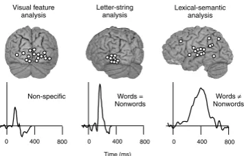
Fig. 5. Cortical dynamics of silent reading. Dots represent centres of active cortical patches collected from individual subjects. The curves display the mean time course of activation in the depicted source areas. Visual feature analysis in the occipital cortex (!100 ms) is stimulus non-specific. The stimulus content starts to matter by!150 ms when activation reflecting letter-string analysis is observed in the left occipitotemporal cortex. Subsequent activation of the left superior temporal cortex at!200–600 ms reflects lexical-semantic analysis and, probably, also phonological analysis. Modified fromSalmelin et al. (2000a).

! Lipp incott W illiams & Wilkins 2000

R. Salmelin / Clinical Neurophysiology xxx (2006) xxx–xxx 5

ARTICLE IN PRESS

Please cite this article as: Riitta Salmelin, Clinical neurophysiology of language: The MEG approach, Clinical Neurophysiology (2006), doi:10.1016/j.clinph.2006.07.316

Figure 1: Cortical dynamics of silent reading. This figure is adapted from (Salmelin, 2007). Dots represent projected sources of activity in the visual cortex (left brain sketch) and the temporal cortex (right brain sketch). The curves display the mean time course of activation in the depicted source ar-eas for different conditions. The initial visual feature anal-ysis in the visual cortex at∼100 ms is non-specific to lan-guage. Comparing responses to letter strings and other vi-sual stimuli reveals that letter string analysis occurs around 150 ms. Finally comparing the responses to words and non-words (made-up non-words) reveals lexical-semantic analysis in the temporal cortex at∼200-500ms.

the context. We set out to find the brain analogs of these model constituents using an MEG decod-ing task. We compare the different models and their representations in terms of how well they can be used to decode the word being read from MEG data. We obtain correspondences between the models and the brain data that are consistent with a model of language processing in which brain activity encodes story context, and where each new word generates additional brain activity, flowing generally from visual processing areas to more high level areas, culminating in an updated story context, and reflecting an overall magnitude of neural effort influenced by the probability of that new word given the previous context.

1.1 Neural processes involved in reading

Humans read with an average speed of 3 words per second. Reading requires us to perceive in-coming words and gradually integrate them into a representation of the meaning. As words are read, it takes 100ms for the visual input to reach the visual cortex. 50ms later, the visual input is processed as letter strings in a specialized region of the left visual cortex (Salmelin, 2007). Be-tween 200-500ms, the word’s semantic properties are processed (see Fig. 1). Less is understood about the cortical dynamics of word integration, as multiple theories exist (Friederici, 2002; Hagoort, 2003).

Magnetoencephalography (MEG) is a brain-imaging tool that is well suited for studying

lan-guage. MEG records the change in the magnetic field on the surface of the head that is caused by a large set of aligned neurons that are changing their firing patterns in synchrony in response to a stimulus. Because of the nature of the signal, MEG recordings are directly related to neural ac-tivity and have no latency. They are sampled at a high frequency (typically1kHz) that is ideal for tracking the fast dynamics of language processing. In this work, we are interested in the mecha-nism of human text understanding as the meaning of incoming words is fetched from memory and integrated with the context. Interestingly, this is analogous to neural network models of language that are used to predict the incoming word. The mental representation of the previous context is analogous to the latent layer of the neural network which summarizes the relevant context before see-ing the word. The representation of the meansee-ing of a word is analogous to the embedding that the neural network learns in training and then uses. Finally, one common hypotheses is that the brain integrates the word with inversely proportional ef-fort to how predictable the word is (Frank et al., 2013). There is a well studied response known as the N400 that is an increase of the activity in the temporal cortex that has been recently shown to be graded by the amount of surprisal of the incoming word given the context (Frank et al., 2013). This is analogous to the output probability of the incom-ing word from the neural network.

Fig. 2 shows a hypothetical activity in an MEG sensor as a subject reads a story in our experi-ment, in which words are presented one at a time for 500ms each. We conjecture that the activity in time windowa, i.e. before wordiis understood, is mostly related to the previous context before see-ing wordi. We also conjecture that the activity in time windowbis related to understanding wordi

and integrating it into the context, leading to a new representation of context in windowc.

Harry'

Harry'

had'

had'

never'

never'

embedding(iC1)' embedding(i)' embedding(i+1)'

context(iC1)'

context(iC2)' context(i)'

out.'prob.(iC1)' out.'prob.(i)' out.'prob.(i+1)'

Studying'the'construc<on'of'meaning'

3' word i+1 word i-1 word i

0.5's'

0.5's' 0.5's'

a b

c

Leila'Wehbe'

'…''Harry'''''''had''''''''never'…''

Figure 2: [Top] Sketch of the updates of a neural network reading chapter 9 after it has been trained. Every word cor-responds to a fixed embedding vector (magenta). A context vector (blue) is computed before the word is seen given the previous words. Given the context vector, the probability of every word can be computed (symbolized by the histogram in green). We only use the output probability of the actual word (red circle). [Bottom] Hypothetical activity in an MEG sensor when the subject reads the corresponding words. The time periods approximated as a, b and c can be tested for in-formation content relating to: the context of the story before seeing wordi(modeled by the context vector ati), the repre-sentation of the properties of wordi(the embedding of word

i) and the integration of wordiinto the context (the output probability of wordi). The periods drawn here are only a conjecture on the timings of such cognitive events.

use the brain data to shed light on what the neural network vectors are representing.

Related work

Decoding cognitive states from brain data is a recent field that has been growing in popularity. Most decoding studies that study language use functional Magnetic Resonance Imaging (fMRI), while some studies use MEG. MEG’s high tempo-ral resolution makes it invaluable for looking at the dynamics of language understanding. (Sudre et al., 2012) decode from MEG the word a subject is reading. The authors estimate from the MEG data the semantic features of the word and use these as an intermediate step to decode what the word is. This is in principle similar to the classification

ap-proach we follow, as we will also use the feature vectors as an intermediate step for word classifica-tion. However the experimental paradigm in (Su-dre et al., 2012) is to present to the subjects sin-gle isolated words and to find how the brain rep-resents their semantic features; whereas we have a much more complex and “naturalistic” experiment in which the subjects read a non-artificial passage of text, and we look at processes that exceed in-dividual word processing: the construction of the meanings of the successive words and the predic-tion/integration of incoming words.

In (Frank et al., 2013), the amount of surprisal that a word has given its context is used to pre-dict the intensity of the N400 response described previously. This is the closest study we could find to our approach. This study was concerned with analyzing the brain processes related only to sur-prisal while we propose a more integral account of the processes in the brain. The study also didn’t address the major contribution we propose here, which is to shed light on the inner constituents of language models using brain imaging.

1.2 Recurrent and finite context neural networks

w(t) s(t−1)

y(t) c(t)

hidden

s(t) output

P(wt+1|s(t))

D W

D0 _X

Figure 3:Recurrent neural network language model.

Recurrent Neural Network Language Model

Unlike standard feedforward neural language models that only look at a fixed number of past words, recurrent neural network language models use all the previous history from position1tot−1

to predict the next word. This is typically achieved by feedback connections, where the hidden layer activations used for predicting the word in posi-tion t−1are fed back into the network to com-pute the hidden layer activations for predicting the next word. The hidden layer thus stores the history of all previous words. We use the RNNLM archi-tecture as described in Mikolov (2012), shown in Figure 3. The input to the RNNLM at positiont

are the one-hot representation of the current word,

w(t), and the activations from the hidden layer at positiont−1,s(t−1). The output of the hidden layer at positiont−1is

s(t) =φ(Dw(t) +Ws(t−1)),

whereDis the matrix of input word embeddings,

Wis a matrix that transforms the activations from the hidden layer in position t − 1, and φ is a sigmoid function, defined as φ(x) = 1

1+exp(−x), that is applied elementwise. We need to compute the probability of the next word w(t+ 1) given the hidden states(t). For fast estimation of out-put word probabilities, Mikolov (2012) divides the computation into two stages: First, the probability distribution over word classes is computed, after which the probability distribution over the subset of words belonging to the class are computed. The class probability of a particular class with indexm

at positiontis computed as:

P(cm(t)|s(t)) = P_Cexp (s(t)Xvm) c=1(exp (s(t)Xvc))

,

whereXis a matrix of class embeddings andvm

is a one-hot vector representing the class with in-dex m. The normalization constant is computed

u1 u2

input words

input embeddings

hidden

h1

hidden

h2

output

P(w|u)

D0

M

C1 _C2

D

Figure 4:Neural probabilistic language model

over all classes C. Each class specifies a subset

V0_{of words, potentially smaller than the entire}

vo-cabularyV. The probability of an output wordlat positiont+ 1 given that its class ism is defined as:

P(yl(t+ 1)|cm(t),s(t)) =

exp (s(t)D0_vl) P_V0

k=1(exp (s(t)D0vk)), whereD0 _{is a matrix of output word embeddings}

andvl is a one hot vector representing the word with indexl. The probability of the wordw(t+ 1)

given its classcican now be computed as:

P(w(t+ 1)|s(t)) =P(w(t+ 1)|ci,s(t))

P(ci|s(t)).

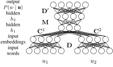
Neural Probabilistic Language Model

We use the feedforward neural probabilistic lan-guage model architecture of Vaswani et al. (2013), as shown in Figure 4. Each contextu comprises a sequence of wordsuj (1 ≤ j ≤ n−1) repre-sented as one-hot vectors, which are fed as input to the neural network. At the output layer, the neu-ral network computes the probabilityP(w|u)for each wordw, as follows.

The output of the first hidden layerh1is

h1=φ

 nX−1

j=1

CjDuj+b1

 _,

the hidden layersh1andh2, which use the activa-tion funcactiva-tionφ(x) = max(0, x).

The output of the second layerh2 is

h2=φ(Mh1+b2),

where M is a weight matrix between h1 and h2 andb2is a vector of biases forh2. The probabil-ity of the output word is computed at the output softmax layer as:

P(w|u) = exp vwD0h2+bTvw

P_V

w0₌₁exp (vw0D0h₂+bTv_w0),

where D0 _{is the matrix of output word}

embed-dings,bis a vector of biases for every output word andvw its the one hot representation of the word

win the vocabulary.

2 Methods

We describe in this section our approach. In sum-mary, we trained the neural network models on a Harry Potter fan fiction database. We then ran these models on chapter 9 ofHarry Potter and the Sorcerer’s Stone (Rowling, 2012) and computed the context and embedding vectors and the output probability for each word. In parallel, 3 subjects read the same chapter in an MEG scanner. We build models that predict the MEG data for each word as a function of the different neural network constituents. We then test these models with a classification task that we explain below. We de-tect correspondences between the neural network components and the brain processes that under-lie reading in the following fashion. If using a neural network vector (e.g. the RNNLM embed-ding vector) allows us to classify significantly bet-ter than chance in a given region of the brain at a given time (e.g. the visual cortex at time 100-200ms), then we can hypothesize a relationship between that neural network constituent and the time/location of the analogous brain process.

2.1 Training the Neural Networks

We used the freely available training tools pro-vided by Mikolov (2012)1 _{and Vaswani et al.}

(2013)2 _{to train our RNNLM and NPLM models}

used in our brain data classification experiments. Our training data comprised around67.5 million

1_{http://rnnlm.org/}

2_{http://nlg.isi.edu/software/nplm}

words for training and100thousand words for val-idation from the Harry Potter fan fiction database (http://harrypotterfanfiction.com). We restricted the vocabulary to the top 100 thousand words which covered all but4 words from Chapter 9 of Harry Potter and the Sorcerer’s Stone.

For the RNNLM, we trained models with differ-ent hidden layers and learning rates and found the RNNLM with 250 hidden units to perform best on the validation set. We extracted our word embed-dings from the input matrixD(Figure 3). We used the default settings for all other hyper parameters. We trained 3-gram and 5-gram NPLMs with 150 dimensional word embeddings and experi-mented with different number of units for the first hidden layer (h1 in Figure 4), and different learn-ing rates. For both the3-gram and 5-gram mod-els, we found750hidden units to perform the best on the validation set and chose those models for our final experiments. We used the output word embeddings D0 _{in our experiments. We visually}

inspected the nearest neighbors in the150 dimen-sional word embedding space for some words and didn’t find the neighbors fromD0 _{orDto be}

dis-tinctly better than each other. We leave the com-parison of input and output embeddings on brain activity prediction for future work.

2.2 MEG paradigm

We recorded MEG data for three subjects (2 fe-males and one male) while they read chapter 9 ofHarry Potter and the Sorcerer’s Stone (Rowl-ing, 2012). The participants were native English speakers and right handed. They were chosen to be familiar with the material: we made sure they had read the Harry Potter books or seen the movies series and were familiar with the characters and the story. All the participants signed the consent form, which was approved by the University of Pittsburgh Institutional Review Board, and were compensated for their participation.

The words of the story were presented in rapid serial visual format (Buchweitz et al., 2009): words were presented one by one at the center of the screen for 0.5 seconds each. The text was shown in 4 experimental blocks of∼11 minutes. In total, 5176 words were presented. Chapter 9 was presented in its entirety without modifications and each subject read the chapter only once.

record the magnetic activity. Our MEG recordings were acquired on an Elekta Neuromag device at the University of Pittsburgh Medical Center Pres-byterian Hospital. This machine has 306 sensors distributed into 102 locations on the surface of the subject’s head. Each location groups 3 sensors or two types: one magnometer that records the in-tensity of the magnetic field and two planar gra-diometers that record the change in the magnetic field along two orthogonal planes3_.

Our sampling frequency was 1kHz. For prepro-cessing, we used Signal Space Separation method (SSS, (Taulu et al., 2004)), followed by its tempo-ral extension (tSSS, (Taulu and Simola, 2006)).

For each subject, the experiment data consists therefore of a 306 dimensional time series of length∼45 minutes. We averaged the signal in ev-ery sensor into 100ms non-overlapping time bins. Since words were presented for 500ms each, we therefore obtain for every wordp = 306×5 val-ues corresponding to 306 vectors of 5 points.

2.3 Decoding experiment

To find which parts of brain activity are related to the neural network constituents (e.g. the RNNLM context vector), we run a prediction and classifica-tion experiment in a 10-fold cross validated fash-ion. At every fold, we train a linear model to pre-dict MEG data as a function of one of the feature sets, using 90% of the data. On the remaining 10% of the data, we run a classification experiment.

MEG data is very noisy. Therefore, classify-ing sclassify-ingle word waveforms yields a low accuracy, peaking at 60%, which might lead to false nega-tives when looking for correspondences between neural network features and brain data. To reveal informative features, one can boost signal by ei-ther having several repetitions of the stimuli in the experiment and then averaging (Sudre et al., 2012) or by combining the words into larger chunks (We-hbe et al., 2014). We chose the latter because the former sacrifices word and feature diversity.

At testing, we therefore repeat the following 300 times. Two sets of words are chosen ran-domly from the test fold. To form the first set, 20 words are sampled without replacement from the test sample (unseen by the classifier). To form the second set, thekth_{word is chosen randomly from} all words in the test fold having the same length as

3_{In this paper, we treat these three different sensors as} three different dimensions without further exploiting their physical properties.

thekth _{word of the first set. Since every fold of} the data was used 9 times in the training phase and once in the testing phase, and since we use a high number of randomized comparisons, this averages out biases in the accuracy estimation. Classifying sets of 20 words improves the classification accu-racy greatly while lowering its variance and makes it dissociable from chance performance. We com-pare only between words of equal length, to mini-mize the effect of the low level visual features on the classification accuracy.

After averaging out the results of multiple folds, we end up with average accuracies that reveal how related one of the models’ constituents (e.g. the RNNLM context vector) is to brain data.

2.3.1 Annotation of the stimulus text

We have 9 sets of annotations for the words of the experiment. Each setj can be described as a ma-trixFjin which each rowicorresponds to the vec-tor of annotations of wordi. Our annotations cor-respond to the 3 model constituents for each of the 3 models: the hidden layer representation before word i, the output probability of word i and the learned embeddings for wordi.

2.3.2 Classification

In order to align the brain processes and the differ-ent constitudiffer-ents of the differdiffer-ent models, we use a classification task. The task is to classify the word a subject is reading out of two possible choices from its MEG recording. The classifier uses one type of feature in an intermediate classification step. For example, the classifier learns to predict the MEG activity for any setting of the RNNLM hidden layer. Given an unseen MEG recording for an unknown wordiand two possible story words

i0_andi00_{(one of which being the true wordi), the}

classifier predicts the MEG activity when reading

i0 _andi00 _{from their hidden layer vectors. It then}

assigns the label i0 _ori00 _{to the word recording i}

depending on which prediction is the closest to the recording. The following are the detailed steps of this complex classification task. However, for the rest of the paper the most useful point to keep in mind is that the main purpose of the classification is to find a correspondence between the brain data and a given feature setj.

2. Divide the data into 10 folds, for each foldb: (a) IsolateMb _andFb

j as test data. The re-mainderM−b_andF−b

j will be used for training4_.

(b) Subtract the mean of the columns of

M−b _fromMb _andM−b _{and the mean} of the columns ofF−b

j fromFbjandF−jb (c) Use ridge regression to solve

M−b_=F−b j ×βtj

by tuning theλparameter to every one of the p output dimensions indepen-dently.λis chosen via generalized cross validation (Golub et al., 1979).

(d) Perform a binary classification. Sample from the set of words inba setcof 20 words. Then sample frombanother set of 20 words such that thekth _{word inc} and dhave the same number of letters. For every sample (c,d):

i. predict the MEG data forcanddas:

Pc_=Fc

j×ΓbjandPd=Fdj ×Γbj ii. assign toMc_{the labelcord}

depend-ing on which ofPc_orPd_{is closest} (Euclidean distance).

iii. assign to Md _{the label c or d} de-pending on which of Pc _{or P}d _is closest (Euclidean distance). 3. Compute the average accuracy.

2.3.3 Restricting the analysis spatially: a searchlight equivalent

We adapt the searchlight method (Kriegeskorte et al., 2006) to MEG. The searchlight is a discovery procedure used in fMRI in which a cube is slid over the brain and an analysis is performed in each location separately. It allows to find regions in the brain where a specific phenomenon is occurring. In the MEG sensor space, for every one of the 102 sensor locations`, we assign a group of sensorsg`. For every location`, we identify the locations that immediately surround it in any direction (Anterior, Right Anterior, Right etc...) when looking at the 2D flat representation of the location of the sensors in the MEG helmet (see Fig. 9 for an illustration of the 2D helmet).g`therefore contains the 3 sensors at location`and at the neighboring locations. The maximum number of sensors in a group is3×9.

4_{The rows fromM}−b_andF−b

j that correspond to the five words before or after the test set are ignored in order to make the test set independent.

The locations at the edge of the helmet have fewer sensors because of the missing neighbor locations.

2.3.4 Restricting the analysis temporally

Instead of using the entire time course of the word, we can use only one of the corresponding 100ms time windows. Obtaining a high classification ac-curacy using one of the time windows and feature setjmeans that the analogous type of information is encoded at that time.

2.3.5 Classification accuracy by time and region

The above steps compute whole brain accuracy us-ing all the time series. In order to perform a more precise spatio-temporal analysis, one can use only one time windowmand one location`for the clas-sification. This can answer the question of when and where different information is represented by brain activity. For every location, we will use only the columns corresponding to the time pointmfor the sensors belonging to the groupg`. Step (d) of the classification procedure is changed as such: (d) Perform a binary classification. Sample from

the set of words inba setcof 20 words. Then sample from b another set of 20 words such that the kth _{word in c and d have the same} number of letters. For every sample (c,d), and for every setting of{m, `}:

i. predict the MEG data for c and d as:

Pc

{m,`} =Fcj×Γbj,{m,`}and

Pd

{m,`} =Fdj ×Γbj,{m,`}

ii. assign toMc

{m,`} the labelcord

depend-ing on which ofPc

{m,`} orPd{m,`} is

clos-est (Euclidean distance). iii. assign toMd

{m,`} the labelcord

depend-ing on which ofPc

{m,`} orPd{m,`} is

clos-est (Euclidean distance).

2.3.6 Statistical significance testing

2014) and inspired by (Chwialkowski and Gret-ton, 2014). For every{m, `}setting we can there-fore compute a standardized z-value by subtract-ing the mean of the shifted classifications and di-viding by the standard deviation. We then com-pute the p-value for the true classification accu-racy being due to chance. Since the three p-values for the three subjects for a given{m, `}are inde-pendent, we combine them using Fisher’s method for independent test statistics (Fisher, 1925). The statistics we obtain for every {m, `} are depen-dent because they comprise nearby time and space windows. We control the false discovery rate us-ing (Benjamini and Yekutieli, 2001) to adjust for the testing at multiple locations and time windows. This method doesn’t assume any kind of indepen-dence or positive depenindepen-dence.

3 Results

We present in Fig. 5 the accuracy using all the time windows and sensors. In Fig. 6 we present the classification accuracy when running the classifi-cation at every time window exclusively. In Fig. 9 we present the accuracy when running the classifi-cation using different time windows and groups of sensors centered at every one of the 102 locations. It is important to lay down some conventions to understand the complex results in these plots. To recap, we are trying to find parallels between model constituents and brain processes. We use:

• a subset of the data (for example the time window 0-100ms and all the sensors)

• one type of feature (for example the hidden context layer from the NPLM 3g model) and we obtain a classification accuracyA. IfA

is low, there is probably no relationship between the feature set and the subset of data. IfAis high, it hints to an association between the subset of data and the mental process that is analogous to the fea-ture set. For example, when using all the sensors and time window 0-100ms, along with the NPLM 3g hidden layer, we obtain an accuracy of 0.70 (higher than chance with p< 10−14_{, see Fig. 6).} Since the NPLM 3g hidden layer summarizes the context of the story before seeing wordi, this sug-gests that the brain is still processing the context of the story before wordibetween 0-100ms.

Fig. 6 shows the accuracy for different types of features when using all of the time points and all the sensors to classify a word. We can see

NPLM 3g NPLM 5g RNNLM

0.6 0.8 1

classification accuracy

hidden layer output probability embeddings

hidden layer output probability embeddings

0.6 0.8 1

classification accuracy

NPLM 3g NPLM 5g RNNLM

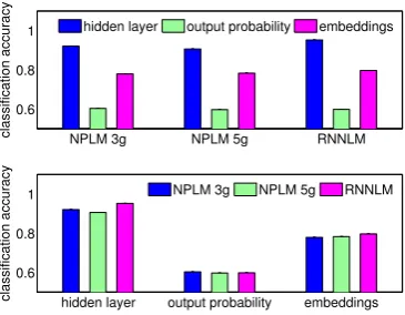
Figure 5: Average accuracy using all time windows and sensors, grouped by model (top) and type of feature (bot-tom). All accuracies are significantly higher than chance (p <10−8_).

0 200 400 0.5

0.6 0.7

NPLM 3g

0 200 400 0.5

0.6 0.7

NPLM 5g

0 200 400 0.5

0.6 0.7

RNNLM

hidden layer output probability embeddings

Figure 6: Average accuracy in different time windows when using different types of features as input to the clas-sifier, for different models. Accuracy is plotted in the center of the respective time window. Points marked with a circle are significantly higher than chance accuracy for the given feature set and time window after correction.

similar classification accuracies for the three types of models, with RNNLM ahead for the hidden layer and embeddings and behind for the output probability features. The hidden layer features are the most powerful for classification. Between the three types of features, the hidden layer fea-tures are the best at capturing the information con-tained in the brain data, suggesting that most of the brain activity is encoding the previous context. The embedding features are the second best. Fi-nally the output probability have the smallest ac-curacies. This makes sense considering that they capture much less information than the other two high dimensional descriptive vectors, as they do not represent the complex properties of the words, only a numerical assessment of their likelihood.

windows starting at 0,100. . .400ms after word presentation. We can see that using the embed-ding vector becomes increasingly more useful for classification until 300-400ms, and then its perfor-mance starts decreasing. This results aligns with the following hypothesis: the word is being per-ceived and understood by the brain gradually after its presentation, and therefore the brain represen-tation of the word becomes gradually similar to the neural network representation of the word (i.e. the embedding vector). The output probability feature accuracy peaks at a later time than the embeddings accuracy. Obtaining a higher than chance accu-racy at time windowmusing the output probabil-ity as input to the classifier suggests strongly that the brain is integrating the word at time window

m, because it is responding differently for pre-dictable and unprepre-dictable words5_{. The}

integra-tion step happens after the percepintegra-tion step, which is probably why the output probability curves peak later than the embeddings curves.

−500 0 500 1000 0.5

0.6 0.7 0.8

Hidden Layer

NPLM 3G NPLM 5G RNNLM

Figure 7:Average accuracy in time for the different hidden layers. The analysis is extended to the time windows before and after the word is presented, the input feature is restricted to be the hidden layer before the central word is seen. The first vertical bar indicates the onset of the word, the second one indicates the end of its presentation.

−1000 0 1000 0.6

0.8

Subject 1

−1000 0 1000 0.6

0.8

Subject 2

−1000 0 1000 0.6

0.8

Subject 3

hidden layer output probability embeddings

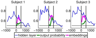
Figure 8: Accuracy in time when using the RNNLM fea-tures for each of the three subjects.

To understand the time dynamics of the hidden layer accuracy we need to see a larger time scale than the word itself. The hidden layer captures the

5_{the fact that we can classify accurately during windows} 300-400ms indicates that the classifier is taking advantage of the N400 response discussed in the introduction

context before wordiis seen. Therefore it seems reasonable that the hidden layer is not only related to the activity when the word is on the screen, but also related to the activity before the word is pre-sented, which is the time when the brain is inte-grating the previous words to build that context. On the other hand, as the word iand subsequent words are integrated, the context starts diverging from the context of wordi(computed before see-ing word i). We therefore ran the same analysis as before, but this time we also included the time windows before and after wordi in the analysis, while maintaining the hidden layer vector to be the context before wordiis seen. We see the behav-ior we predicted in the results: the context before seeing wordibecomes gradually more useful for classification until wordiis seen, and then it grad-ually decreases until it is no longer useful since the context has changed. We observe the RNNLM hidden layer has a higher classification accuracy than the finite context NPLMs. This might be due to the fact that the RNNLM has a more complete representation of context that captures more of the properties of the previous words.

To show the consistency of the results, we plot as illustration the three curves we obtain for each subject for the RNNLM (Fig. 8). The patterns seem very consistent indicating the phenomena we described can be detected at the subject level.

Back%

hidden layer output probability embeddings

0 500 0.5 0.6 0.7

time (s)

accuracy

Le(% Right%

hidden layer output probability embeddings

0 500

0.5 0.6 0.7

time (s)

accuracy

hidden layer output probability embeddings

0 500

0.5 0.6 0.7

time (s)

accuracy

hidden layer

output probability

embeddings

0

500

0.5

0.6

0.7

time (s)

accuracy

hidden layer

output probability

embeddings

0

500

0.5

0.6

0.7

time (s)

accuracy

hidden layer

output probability

embeddings

0

500

0.5

0.6

0.7

time (s)

accuracy

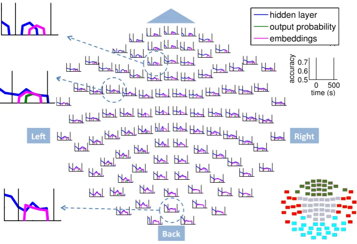
Figure 9: Average accuracy in time and space on the MEG helmet when using the RNNLM features. For each of the 102 locations the average accuracy for the group of sensors centered at that location is plotted versus time. The axes are defined in the rightmost, empty plot. Three plots have been magnified to show the increasing delay in high accuracy when using the embeddings feature, reflecting the delay in processing the incoming word as information travels through the brain. A sensor map is provided in the lower right corner: visual cortex = cyan, temporal = red, frontal = dark green.

is reported in the literature. Finally, as we reach the frontal cortex, we see that the embeddings fea-tures have an even later accuracy peak.

4 Conclusion and contributions

Novel brain data exploration We present here

a novel and revealing approach to shed light on the brain processes involved in reading. This is a departure from the classical approach of control-ling for a few variables in the text (e.g. showing a sentence with an expected target word versus an unexpected one). While we cannot make clear cut causal claims because we did not control for our variables, we are able to explore the data much more and offer a much richer interpretation than is possible with artificially constrained stimuli.

Comparing two models of language Adding

brain data into the equation allowed us to com-pare the performance of the models and to identify a slight advantage for the RNNLM in capturing the text contents. Numerical comparison is how-ever a secondary contribution of our approach. We showed that it might be possible to use brain data to understand, interpret and illustrate what exactly is being encoded by the obscure vectors that neural networks compute, by drawing parallels between the models constituents and brain processes.

Anecdotally, in the process of running the ex-periments, we noticed that the accuracy for the hidden layer of the RNNLM was peaking in the time window corresponding to wordi−2, and that it was decreasing during word i−1. Since this was against our expectations, we went back and looked at the code and found that it was indeed returning a delayed value and corrected the fea-tures. We therefore used the brain data in order to correct a mis-specification in our neural network model. This hints if not proves the potential of our approach for assessing language models.

Future Work The work described here is our

first attempt along the promising endeavor of matching complex computational models of lan-guage with brain processes using brain recordings. We plan to extend our efforts by (1) collecting data from more subjects and using various types of text and (2) make the brain data help us with training better statistical language models by using it to de-termine whether the models are expressive enough or have reached a sufficient degree of convergence.

Acknowledgements

References

Yoav Benjamini and Daniel Yekutieli. 2001. The con-trol of the false discovery rate in multiple testing un-der dependency. Annals of statistics, pages 1165– 1188.

Augusto Buchweitz, Robert A Mason, Lˆeda Tomitch, and Marcel Adam Just. 2009. Brain activation for reading and listening comprehension: An fMRI study of modality effects and individual differences in language comprehension. Psychology & neuro-science, 2(2):111–123.

Kacper Chwialkowski and Arthur Gretton. 2014. A kernel independence test for random processes.

arXiv preprint arXiv:1402.4501.

Ronald Aylmer Fisher. 1925. Statistical methods for research workers. Genesis Publishing Pvt Ltd. Stefan L Frank, Leun J Otten, Giulia Galli, and

Gabriella Vigliocco. 2013. Word surprisal predicts N400 amplitude during reading. InProceedings of the 51st annual meeting of the Association for Com-putational Linguistics, pages 878–883.

Angela D Friederici. 2002. Towards a neural basis of auditory sentence processing. Trends in cognitive sciences, 6(2):78–84.

Gene H Golub, Michael Heath, and Grace Wahba. 1979. Generalized cross-validation as a method for choosing a good ridge parameter. Technometrics, 21(2):215–223.

Peter Hagoort. 2003. How the brain solves the binding problem for language: a neurocomputational model of syntactic processing.Neuroimage, 20:S18–S29. Nikolaus Kriegeskorte, Rainer Goebel, and Peter

Ban-dettini. 2006. Information-based functional brain mapping. Proceedings of the National Academy of Sciences of the United States of America, 103(10):3863–3868.

Tomas Mikolov, Stefan Kombrink, Anoop Deoras, Lukar Burget, and J Cernocky. 2011. RNNLM-recurrent neural network language modeling toolkit. In Proc. of the 2011 ASRU Workshop, pages 196– 201.

Tomas Mikolov. 2012. Statistical Language Models Based on Neural Networks. Ph.D. thesis, Brno Uni-versity of Technology.

Vinod Nair and Geoffrey E. Hinton. 2010. Rectified linear units improve restricted Boltzmann machines. InProceedings of ICML, pages 807–814.

Joanne K. Rowling. 2012. Harry Potter and the Sor-cerer’s Stone. Harry Potter US. Pottermore Limited. Riitta Salmelin. 2007. Clinical neurophysiology of language: the MEG approach. Clinical Neurophysi-ology, 118(2):237–254.

Gustavo Sudre, Dean Pomerleau, Mark Palatucci, Leila Wehbe, Alona Fyshe, Riitta Salmelin, and Tom Mitchell. 2012. Tracking neural coding of percep-tual and semantic features of concrete nouns. Neu-roImage, 62(1):451–463.

Samu Taulu and Juha Simola. 2006. Spatiotem-poral signal space separation method for rejecting nearby interference in MEG measurements. Physics in medicine and biology, 51(7):1759.

Samu Taulu, Matti Kajola, and Juha Simola. 2004. Suppression of interference and artifacts by the sig-nal space separation method. Brain topography, 16(4):269–275.

Ashish Vaswani, Yinggong Zhao, Victoria Fossum, and David Chiang. 2013. Decoding with large-scale neural language models improves translation. Leila Wehbe, Brian Murphy, Partha Talukdar, Alona