Abstract— We proposed an algorithm for predicting friction coefficient from visual information for mobile robot since coefficient of friction is very important in driving on road and traversing over obstacle. Our algorithm is based on terrain classification for visual image. To predict friction coefficient from given image, we divide an image into homogeneous regions which have same material composition. The proposed method, non-contacting approach, has advantage over other methods that extract material characteristic of road by sensors contacting road surface. Obtaining information about friction coefficient before entering such terrain can be very useful for path planning and avoiding slippery areas. And we form a group of each terrain type. So, when new terrain is entered into a system, the data of new terrain are classified into each group. By grouping each terrain to use the same regression coefficients, we can reduce the amount of processing time. The proposed method will be verified by real outdoor environment with real vehicles.
Index Terms— Mobile robot, Path planning, Unmanned vehicle, Vision sensor.
I. INTRODUCTION
Autonomous mobile robots are increasingly required to operate in unstructured environments. A fundamental requirement for systems in such environments is the capacity to accurately negotiate friction coefficient of road surface. Friction coefficient is very important in driving on road or human drivers as well as autonomous mobile robots. The goal of predicting friction coefficient is to support safe navigation in outdoor environments. Due to the rich variety of ground surfaces, it is important for the robot to know the type of the forthcoming terrain, as each terrain poses different possible hazards to the robot [1]. The mobility of a vehicle on off-road terrain is known to be strongly influenced by the interaction between the vehicle and the terrain. Also, kinematics and dynamics of mobile robots should be Manuscript received July 26, 2009. Authors are gratefully acknowledging the financial support by Agency for Defence Development and by UTRC(Unmanned Technology Research Center).
Doogyu Kim is with the BK21 Mechatronics Group at Chungnam National University, Daejeon, Republic of Korea (e-mail: doogie@ cnu.ac.kr).
Jayoung Kim is with the BK21 Mechatronics Group at Chungnam National University, Daejeon, Republic of Korea (e-mail: [email protected])
Jihong Lee is with the BK21 Mechatronics Group at Chungnam National University, Daejeon, Republic of Korea (phone: +82-42-821-6873; fax: +82-42-823-4919; e-mail:[email protected]).
Hanbyul Joo is with Korea Advanced Institute of Science and Technology, Daejeon, Republic of Korea, (e-mail: [email protected])
In-so Kweon is with Korea Advanced Institute of Science and Technology, Daejeon, Republic of Korea, (e-mail: [email protected]).
considered to apply traction control technology for overcoming rough terrain [2,3].
The friction coefficients are known to be dependent on terrain characteristics which are determined compositional materials such as soil, small gravel, gravel, and asphalt. So, the first thing for autonomous mobile robot to travel along arbitrary terrain is to classify the terrain.
Terrain classification methods provide semantic descriptions of physical property of a given terrain. These descriptions can be associated with nominal numerical physical parameters, and/or nominal traversability estimates, to improve accuracy in predicting traversability. Numerous researchers have proposed terrain classification methods based on features derived from remote sensor data such as color and image texture [4,5,6]. Most of these algorithms have been developed in the context of terrestrial unmanned ground vehicles where the visual features have wide variance [7].
In this paper we proposed a method for for predicting friction coefficient from a terrain image so that robot can react to environmental change. To simplify this problem, we don’t take geometric information into consideration rather than material information. Visual characteristic of the terrain, in addition to material characteristics, can give more clues to its mechanical properties and the eventual terrain interaction. Thus, we propose to use vision data as input for friction coefficient prediction [8].
Our method is executed as follows. At first, we use texture based classification method to extract material information from each area (later we call it “segment”) of image of environment. Because some homogenous terrains have not uniform geometrical shape but similar color, our approach is feasible for this case. Leung and Malik defined a concept of texton in operational manner [9]. This method used texture based classification method to make super-pixel. By using his segmentation technique, we divide an image into homogeneous regions which have similar colors. In advance, a set of learning images are collected to classify the characteristics of each segment. By comparing a given segment with every learning image, we obtain compositional ratio of materials. This result is terrain information.
We will group each terrain by using compositional ratio of materials of terrains. The groups are useful in time saving when new image which is different from learning image is going to be classified. Using probability theory, the data of new image is classified into each group. Thus, we can apply to predict friction coefficient usefully.
The input for predicting friction coefficient (i.e. the terrain information) will be represented by the compositional ratio of materials of the facing position of the autonomous mobile
Utilizing Visual Information for Path Planning of
Autonomous Mobile Robot
robot. Path planning of autonomous mobile robot depends on the predicted result so as to avoid slippery area.
II. OVER-SEGMENTATION METHOD
In this section we describe the over-segmentation method using vision information. We use Leung and Malik’s filter bank to get filter response. Their method showed that many textures could be represented and be recreated using a small number of basis vectors extracted from the local descriptors; they called the basis vectors textons. Also, we then generate texton histogram using all filter response of training images. In this case, we use Verma’s method [10] because it is much simple.
[image:2.595.317.535.101.261.2]Over-segmentation algorithm divides image into homogenous regions which have homogenous material for making super-pixels and classifying. And we decided to adopt over-segmentation method of Felzenszwalb et al.[11]. This over-segmentation method generates good result in merging similar pixel to one segment [12] Fig. 1 shows sample image of terrain before over-segmentation.
Fig. 1. Sample image of terrain
In the fig. 2, the pixels of each segment have almost similar color. So, we can assume that each segment is composed of same material composition. Actually, there are some regions which is divided different segment even if they are same material. However, it does not matter because we can predict they can be classified into same material at classifying step.
Fig. 2. Over-segmentation result of sample image.
We use learning image for acquiring compositional ratio of material in each segment. Therefore we collect learning images of each material for texture recognition technique. Six materials (sky, soil, small gravel, gravel, forest, and
[image:2.595.88.262.323.466.2]asphalt) compose learning images. Fig. 3 shows learning image. Learning image is rectangular and it is different in size.
Fig. 3. Selected image segment for learning (sky, soil, small gravel, gravel, forest, and asphalt)
Each segment is compared with learning images to give out compositional ratio of material for the segment. This result of comparison is terrain information and it is in requisition prediction method. Histogram in fig. 4 shows terrain information.
Fig. 4. Histogram of compositional ratio of material (terrain information
III. PREDICTION METHOD
In this section we describe prediction system for path planning of autonomous mobile robot. This method classify new image into group. And it predict friction coefficient of new image.
A. Grouping terrains and classifying new terrain
[image:2.595.311.544.377.511.2] [image:2.595.89.260.575.708.2](1) to fit best the distribution of each group. ) ( 1 ) ( 2 1 ) det( 2 1 ) ( ) , ( μ μ π μ − − Σ − − Σ = Σ X T X e d X g (1) T : Transpose matrix
d : Dimension of data
Here, μ is mean vector of (d×1) which is the center of Gaussian and Σ is covariance matrix of (d×d). Note that d is dimension of data. The Gaussian distribution is important to group the data of each image.
To classify new image into different groups, Maximum Likelihood Estimation (MLE) and Bayesian classification are used. We briefly describe the idea in the following.
) | ( 1 ) |
( θ P XK θ
n k X P = Π = (2)
∑
= = ∧ n k k X n 1 1 μ (3)∑
= ∧ − ∧ − = ∧ Σ n k T k X k X n 1 ) )( (1 μ μ
(4) n : The number of segments
T : Transpose matrix
As described in equation (2), a sample data set X = ( X1,X2,...,Xn) is observed from a probability density function composed of a parameter set θ = (θ1 ,…, θm ). Here, P(X|θ)is the likelihood function of given data set which depends on a parameterθ. Note that θrepresented sample mean μˆ and sample covariance Σˆ when the probability density function is described as Gaussian distribution as described in equation (3) and (4).
∑
= = c j D i P D i Y P D i P D i Y P D Y i P 1 ) | ( ) , | ( ) | ( ) , | ( ) , | ( ω ω ω ω ω (5)c : The number of data of new image
Estimated sample mean μˆ and covariance Σˆ form a group of the data of terrain image. The equation (5) is Bayesian classification. Dis the sample data sets of terrain image and ωiis identifier of each group. When new image is captured, Bayesian classification calculates a posterior probability of Y which is 2-dimensional data of the new image. Thus, the data of new image is classified into specified group ωiof the prior terrain image which has the most high posterior probability value.
B. Setting up Prediction function
Prediction function requires regression coefficients. Equation (6) is cost function for computing of regression coefficient. This cost function compute regression coefficient
from terrain information of one group. Thus each group have different regression coefficient. Our cost function can be written in the following form:
∑∑
= = > < + − C c N i i c c c c i i bbc c c F K x x b b x x
1 1 2 1 0 , , { ( , )[ , ]} min 1 0 λ (6) i
F
: Corresponding measurements of friction coefficient at segmenti
x
: Terrain informationc
x
: Training exampleN
: The number of terrain information in one groupC
: The number of training examplesc c
b
b
0,
1 : Regression coefficientswhere K(xi,xc) is a weight function, K(x,xc)=exp(−||x−xc||2/λ),
and the
λ
which determines the receptive fields size.C. Predicting newly given data
New terrain information is classified into the most similar group by grouping method. This group have regression coefficient. It is in requisition prediction function. Prediction function compute friction coefficient of entered new terrain. Our prediction function written in the following from:
∑
= ∧ > < + = C c c c cc b b x x
x x K x
F
1 10 , )
)( , ( )
( (7)
where
x
are compositional ratio of material of new terrain, and∧
Fis friction coefficient of new terrain.
IV. EXPERIMENTAL RESULT
In this section we give experimental results of predicting friction coefficient from terrain information. This section describes experiment equipment. Also, it obtains grouping new terrain and classifying new terrain. The last of section describes result of prediction function.
A. Experiment equipment
Fig. 5. Experiment for measurement of friction coefficient Traction car pulls experimental vehicle. At the instance when the experimental vehicle starts to slip, we collect the data of Load Cell. The collected data include the information of friction between wheel and ground.
B. Grouping terrains and classifying new terrain
[image:4.595.57.278.48.187.2]We considered the images of four terrains which are taken a picture experimentally. Each image is the image of soil, small gravel, gravel, and asphalt terrains. To get a sample data, six frames of four terrain types are used as shown in Fig 5. As previously stated at chapter Ⅲ, Compositional ratio of the terrain image consists of 4-dimentional data (each compositional ratio: soil, small gravel, gravel and asphalt). By PCA, the 4-dimensional data is changed into 2-dimensional data which contain principal information of high dimensional feature vectors. The 2-dimensional data of each terrain make Gaussian distribution by using equation (1). Consequently, the data of terrain images form groups which have mean μ and covariance ∑. Mean μ and covariance ∑ of each terrain are calculated as the following table 1.
Fig. 5 Sample images of four terrains. Soil terrain (top left), small gravel terrain (top right), gravel terrain (bottom left), and asphalt terrain (bottom right).
Table.1 The mean and covariance of each sample
Identifier ωi μi ∑i
Group1 (soil terrain)
μ1 (0.2308, 0.2994)
∑1 ⎥
⎦ ⎤ ⎢
⎣ ⎡ −
− 2857 . 0 3221 . 0
3221 . 0 4198 . 0
×10^-4
Group2
(small gravel terrain )
μ2 (0.3079, 0.2344)
∑2 ⎥
⎦ ⎤ ⎢
⎣ ⎡ −
− 1575 . 0 0408 . 0
0408 . 0 0201 . 0
×10^-2
Group3 (gravel terrain)
μ3 (0.3122, 0.1701)
∑3 ⎥
⎦ ⎤ ⎢
⎣ ⎡ −
− 5160 . 0 2350 . 0
2350 . 0 1815 . 0
×10^-3
Group4
(asphalt terrain)
μ4 (0.1987, 0.0615)
∑4 ⎥
⎦ ⎤ ⎢
⎣ ⎡ −
− 3141 . 0 0937 . 0
0937 . 0 5733 . 0
[image:4.595.307.544.52.439.2]×10^-4
Fig. 6 The grouping result of each terrain
[image:4.595.51.289.498.659.2]Fig 6 shows the grouping result of each terrain. The cross line (+) of each group is mean μ and the shape of each group is formed by covariance ∑.
[image:4.595.311.508.522.669.2]Fig. 8 The new image of asphalt terrain
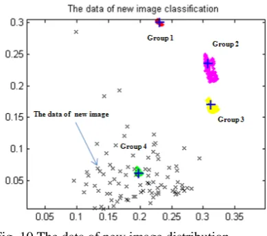
[image:5.595.311.542.226.370.2]When the data sets of new terrain image as shown in Fig 7, 8 are entered into a system, also each data of new terrain image is processed as 2-dimensional data by PCA. The data of new image are distributed in Fig 9, 10. As the next processing, the posterior probability of each data of new image are calculated by Bayesian classification which compares each data of new image with Parameter θ=(μˆ,Σˆ)of each group. Consequently, each data is classified by identifier ωi into the group where the posterior probability is the most.
Fig. 9 The data of new image distribution (New image 1 of soil terrain)
Fig. 10 The data of new image distribution (New image 2 of asphalt terrain)
As shown in Table 2, elements of input data set of new image are classified individually. Here, the number of the data is the number of segments of each terrain. Each of all data of terrain image 1 is classified into group 1(69 unit) and group 2 (39 unit). Consequently, we can know that newly entered terrain is close to group 1 “soil terrain”. Also, each of all data of terrain image 2 is classified into group 1(10 unit), group 2 (5 unit), and group 3 (75 unit). Thus, we can know that newly entered terrain is close to group 4 “asphalt terrain”.
[image:5.595.49.252.375.546.2]Each data of new terrain images is classified into one of four groups to process rapidly predicting friction coefficients by using same regression coefficients.
Table.2 The data of new image classification
Identifier ωi New image 1 classification
New image 2 classification
Group1
(soil terrain) 69 segments 10 segments
Group2
(small gravel terrain ) 39 segments 5 segments
Group3
(gravel terrain) 0 segments 0 segments
Group4
(asphalt terrain) 0 segments 75 segments
Classification Result
Group 1 soil terrain
Group 4 asphalt terrain
C. Prediction result of new terrain
Prediction function use regression coefficient in one group. This group includes new terrain. And it have different regression coefficient each segment (Table. 3). Regression coefficient include terrain character each group.
Table.3 Regression coefficient
c
b
0b
c1
Group 1 0.9041 0.2354
Group 2 0.8575 -0.4288
Group 3 0.9487 -0.4835
Group 4 1.1419 -0.529
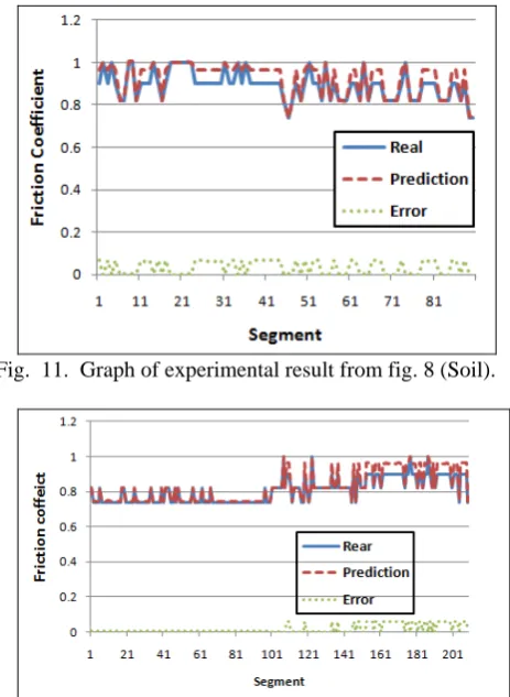
New terrain in fig.7 (Soil) is classified into the group 1 and new terrain in fig. 8 (Asphalt) is classified into the group 4 (Table. 2). Predicting friction coefficient for soil terrain use regression coefficient of group 1 in table. 3, and predicting friction coefficient for asphalt terrain use regression coefficient of group 4 in table. 3.
[image:5.595.300.535.467.552.2] [image:5.595.51.246.583.755.2]Fig. 11. Graph of experimental result from fig. 8 (Soil).
Fig. 12. Graph of experimental result from fig. 9 (Asphalt). Green line (dot) shows error between real friction coefficient and predicting friction coefficient. That is average error by less than 0.035 (friction coefficient). This error is small.
V. CONCLUSION
In this paper we have proposed to predict friction coefficient for path planning of autonomous mobile robot. The idea is to map the material information of the forthcoming terrain. The importance of this method is that it is predictive. That is, the autonomous mobile robot can avoid terrains of large slip before getting stuck. The output of the prediction algorithm is intended to be incorporated into a more intelligent path planning. And we make use of grouping and classify for short time to process. These algorithms form a group similar terrain type.
In the future study, further efforts are needed to develop a better predicting friction coefficient and grouping of terrain, to avoid erroneous prediction algorithm due to prediction system errors.
ACKNOWLEDGMENT
Authors are Gratefully acknowledging the financial support by Agency for Defence Development and by UTRC(Unmanned Technology Research Center)
REFERENCES
[1] Christian Weiss, Hashem Tamini, and Andreas Zell, “A Combination of Vision- and Vibration-based Terrain Classification,” IROS, pp.2204-2209, 2008
[2] Karl Iagnemma, Shinwoo Kang, Hassan Shibl, steven Dubowsky, “Online Terrain Parameter Estimation for Wheeled Mobile Robots With Apllication to Planetary Rovers,” IEEE Transactions on Robotics and Automation, vol.20, no.5, pp.921-927, 2004
[3] Pierre Lamon and Roland Siegwart, “Wheel Torque Control in Rough Terrain-Modeling and Simulation,” In Proceedings of the IEEE international conference on robotics and automation, pp.867-872, 2005 [4] R. Manduchi, A. Castano, A. Talukder and L. Matthies, “Obstacle
Detection and Terrain Classification for Autonomous Off-Road Navigation,” Autonomous Robots 18, Springer, pp.81-102, 2005 [5] Paul Jansen, Wannes van der Mark, Johan C. van den Heuvel, Frans
C.A. Groen, “Colour based Off-Road Environment and Terrain Type Classification,” IEEE Conference on Intelligent Transportation Systems, pp. 61-66, 2005
[6] Morten Rufus Blas, Motilal Agrawal, Aravind Sundaresan and Kurt Konolige, “Fast Color/Texture Segmentation for Outdoor Robots,” IROS, pp. 4078-4085, 2008
[7] Ibrahim Halatci, Christopher A. Brooks, Karl Iagnemma, “Terrain Classification and Classifier Fusion for Planetary Exploration Rovers,” In Proc. IEEE Aerospace Conference, USA, 2007
[8] Anelia Angelova, Larry Matthies and Daniel Helmick, Pietro Perona, “Learning and Prediction of Slip from Visual Information,” Journal of Field Robotics, vol. 24, no. 3, pp.205-231, 2007
[9] T. Leung and J. Malik, “Representing and Recognizing the Visual Appearance of Materials Using the Three-dimensional Texton,” IJCV vol. 43, no. 1, 2001
[10] M. Varma and A. Zisserman, “Classifying images of materials: achieving viewpoint and illumination independence,” ECCV, vol. 3, pp.255-271, 2002
[11] P. Felzenszwalb and D. Huttenlocher, “Efficient Graph based Image Segmentation,” IJCV, vol. 59, no. 2, pp.167-181, 2004