Reverse Engineering of Tree Kernel Feature Spaces
Daniele Pighin FBK-Irst, HLT
Via di Sommarive, 18 I-38100 Povo (TN) Italy
Alessandro Moschitti University of Trento, DISI
Via di Sommarive, 14 I-38100 Povo (TN) Italy
Abstract
We present a framework to extract the most important features (tree fragments) from a Tree Kernel (TK) space according to their importance in the target kernel-based machine, e.g. Support Vector Ma-chines (SVMs). In particular, our min-ing algorithm selects the most relevant fea-tures based on SVM estimated weights and uses this information to automatically infer an explicit representation of the in-put data. The explicit features (a) improve our knowledge on the target problem do-main and (b) make large-scale learning practical, improving training and test time, while yielding accuracy in line with tradi-tional TK classifiers. Experiments on se-mantic role labeling and question classifi-cation illustrate the above claims.
1 Introduction
The last decade has seen a massive use of Support Vector Machines (SVMs) for carrying out NLP tasks. Indeed, their appealing properties such as 1) solid theoretical foundations, 2) robustness to irrelevant features and 3) outperforming accuracy have been exploited to design state-of-the-art lan-guage applications.
More recently, kernel functions, which im-plicitly represent data in some high dimensional space, have been employed to study and fur-ther improve many natural language systems, e.g. (Collins and Duffy, 2002), (Kudo and Matsumoto, 2003), (Cumby and Roth, 2003), (Cancedda et al., 2003), (Culotta and Sorensen, 2004), (Toutanova et al., 2004), (Kazama and Torisawa, 2005), (Shen et al., 2003), (Gliozzo et al., 2005), (Kudo et al., 2005), (Moschitti et al., 2008), (Diab et al., 2008). Unfortunately, the benefit to easily and effectively model the target linguistic phenomena is reduced
by the the implicit nature of the kernel space, which prevents to directly observe the most rele-vant features. As a consequence, even very accu-rate models generally fail in providing useful feed-back for improving our understanding of the prob-lems at study. Moreover, the computational bur-den induced by high dimensional kernels makes the application of SVMs to large corpora still more problematic.
In (Pighin and Moschitti, 2009), we proposed a feature extraction algorithm for Tree Kernel (TK) spaces, which selects the most relevant features (tree fragments) according to the gradient compo-nents (weight vector) of the hyperplane learnt by an SVM, in line with current research, e.g. (Rako-tomamonjy, 2003; Weston et al., 2003; Kudo and Matsumoto, 2003). In particular, we provided al-gorithmic solutions to deal with the huge dimen-sionality and, consequently, high computational complexity of the fragment space. Our experimen-tal results showed that our approach reduces learn-ing and classification processlearn-ing time leavlearn-ing the accuracy unchanged.
In this paper, we present a new version of such algorithm which, under the same parameteriza-tion, is almost three times as fast while produc-ing the same results. Most importantly, we ex-plored tree fragment spaces for two interesting natural language tasks: Semantic Role Labeling (SRL) and Question Classification (QC). The re-sults show that: (a) on large data sets, our ap-proach can improve training and test time while yielding almost unaffected classification accuracy, and (b) our framework can effectively exploit the ability of TKs and SVMs to, respectively, gener-ate and recognize relevant structured features. In particular, we (i) study in more detail the relevant fragments identfied for the boundary classification task of SRL, (ii) closely observe the most relevant fragments for each QC class and (iii) look at the di-verse syntactic patterns characterizing each
tion category.
The rest of the paper is structured as follows: Section 2 will briefly review SVMs and TK func-tions; Section 3 will detail our proposal for the lin-earization of a TK feature space; Section 4 will review previous work on related subjects; Section 5 will detail the outcome of our experiments, and Section 6 will discuss some relevant aspects of the evaluation; finally, in Section 7 we will draw our conclusions.
2 Tree Kernel Functions
The decision function of an SVM is:
f(~x) = ~w·~x+b=Xn
i=1
αiyi~xi·~x+b (1)
where~xis a classifying example and ~wandbare the separating hyperplane’s gradient and its bias, respectively. The gradient is a linear combination of the training points ~xi, their labels yi and their weightsαi. Applying the so-called kernel trick it is possible to replace the scalar product with a ker-nel function defined over pairs of objects:
f(o) =Xn
i=1
αiyik(oi, o) +b
with the advantage that we do not need to provide an explicit mappingφ(·)of our examples in a vec-tor space.
A Tree Kernel function is a convolution ker-nel (Haussler, 1999) defined over pairs of trees. Practically speaking, the kernel between two trees evaluates the number of substructures (or frag-ments) they have in common, i.e. it is a measure of their overlap. The function can be computed re-cursively in closed form, and quite efficient imple-mentations are available (Moschitti, 2006). Dif-ferent TK functions are characterized by alterna-tive fragment definitions, e.g. (Collins and Duffy, 2002) and (Kashima and Koyanagi, 2002). In the context of this paper we will be focusing on the SubSet Tree (SST) kernel described in (Collins and Duffy, 2002), which relies on a fragment defi-nition that does not allow to break production rules (i.e. if any child of a node is included in a frag-ment, then also all the other children have to). As such, it is especially indicated for tasks involving constituency parsed texts.
Implicitly, a TK function establishes a corre-spondence between distinct fragments and dimen-sions in some fragment space, i.e. the space of all
Fragment space
A
B A A
B A
B A A
B A
C A
B A
B A
C A
C D
B A D
B A
C
1 2 3 4 5 6 7
T1
A
B A
B A
C
T2
D
B A
C
φ(T1) = [2,1,1,1,1,0,0]
[image:2.595.314.522.62.211.2]φ(T2) = [0,0,0,0,1,1,1] K(T1, T2) =hφ(T1), φ(T2)i= 1
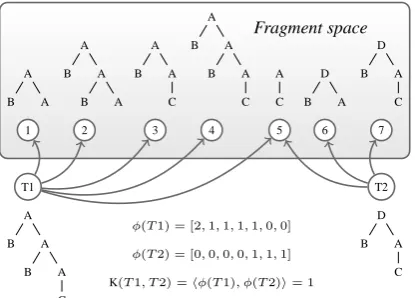
Figure 1: Esemplification of a fragment space and the kernel product between two trees.
the possible fragments. To simplify, a tree t can be represented as a vector whose attributes count the occurrences of each fragment within the tree. The kernel between two trees is then equivalent to the scalar product between pairs of such vectors, as exemplified in Figure 1.
3 Linearization of a TK function
Our objective is to efficiently mine the most rele-vant fragments from the huge fragment space, so that we can explicitly represent our input trees in terms of these fragments and learn fast and accu-rate linear classifiers.
The framework defines five distinct activities, detailed in the following paragraphs.
3.1 Kernel Space Learning (KSL)
The first step involves the generation of an approx-imation of the whole fragment space, i.e. we can consider only the trees that encode the most rele-vant fragments. To this end, we can partition our training data intoSsmaller sets, and use the SVM and the SST kernel to learn S models. We will only consider the fragments encoded by the sup-port vectors of theSmodels. In the next stage, we will use the SVM estimated weights to drive our feature selection process.
Algorithm 3.1: MINE MODEL(M, L, λ)
global maxexp
prev← ∅; CLEAR INDEX()
for eachhαy, ti ∈M
do
Ti←α·y/ktk
for eachn∈ Nt
do
(f←
FRAG(n) ; rel=λ·Ti
prev←prev∪ {f, rel} PUT(f, rel)
best pr←BEST(L) ;
while true
do
next← ∅
for eachhf, reli ∈previff∈best pr
do
X =EXPAND(f, maxexp)
rel exp←λ·rel
for eachfrag∈ X
do
(
temp={frag, rel exp}
next←next∪temp
PUT(frag, rel exp)
best←BEST(L)
if notCHANGED()
then break
best pr←best prev←next
FL←best pr
return(FL)
Nonetheless, since we do not need to employ them for classification (but just to direct our feature se-lection process, as we will describe shortly), we can accept to rely on sub-optimal weights. Fur-thermore, research results in the field of SVM par-allelization using cascades of SVMs (Graf et al., 2004) suggest that support vectors collected from locally learnt models can encode many of the rel-evant features retained by models learnt globally. Henceforth, letMs be the model associated with thes-th split, andFsthe fragment space that can describe all the trees inMs.
3.2 Fragment Mining and Indexing (FMI)
In Equation 1 it is possible to isolate the gradient
~w =Pni=1αiyi~xi, with ~xi = [x(1)i , . . . , x(iN)],N being the dimensionality of the feature space. For a tree kernel function, we can rewritex(ij)as:
x(ij)= ti,jkλtℓ(fj)
ik =
ti,jλℓ(fj)
qPN
k=1(ti,kλℓ(fk))2 (2)
where: ti,j is the number of occurrences of the fragmentfj, associated with thej-th dimension of the feature space, in the treeti;λis the kernel de-cay factor; andℓ(fj)is the depth of the fragment.
The relevance|w(j)|of the fragment fj can be
measured as:
|w(j)|=Xn
i=1
αiyix(ij)
=
Pni=1αiyiti,jλℓ(fj)
ktik .
(3) We fix a threshold L and from each model Ms (learnt during KSL) we select theLmost relevant fragments, i.e. we build the setFs,L=∪k{fk}so that:
|Fs,L|=Land|w(k)| ≥ |w(i)|∀fi ∈ F \ Fs,L.
To generate all the fragments encoded in a model, we adopt the greedy strategy described in Algorithm 3.1. Its arguments are: an SVM model
M represented as hαy, ti pairs, where t is a tree structure; the threshold valueL; and the kernel de-cay factorλ.
The function FRAG(n) generates the smallest fragment rooted in noden(i.e. for an SST kernel, the fragment consisting of n and its direct chil-dren). We call such fragment a base fragment. The function EXPAND(f, maxexp) generates all the
fragments that can be derived from the fragment
f by expanding, i.e. including in the fragment the direct children of some of its nodes. These frag-ments are derived fromf. The parametermaxexp limits fragment proliferation by setting the maxi-mum number of nodes which can be expanded in a fragment expansion operation. For example, if there are 10 nodes which can be expanded in frag-mentf, then only the fragments where at most 3 of the 10 nodes are expanded will be generated by a call toEXPAND(f,3).
Every time we generate a fragmentf, the func-tionPUT(f, rel)saves the fragment along with its relevance rel in an index. The index keeps track of the cumulative relevance of a fragment, and its implementation has been optimized for fast inser-tions and spatial compactness.
A whole cycle of expansions is considered as an iteration of the mining process: we take into account all the fragments that have undergone k expansions and produce all the fragments that re-sult from a further expansion, i.e. all the fragments expandedk+ 1times.
the iteration is complete we re-evaluate the set of
Lbest fragments in the index, and we stop only if the worst of them, i.e. the L-th ranked fragment at the stepk+ 1, and its score are the same as at the end of the previous iteration. That is, we as-sume that if none of the fragments mined during the(k+ 1)-th iteration managed to affect the bot-tom of the pool of theLmost relevant fragments, then none of their expansions is likely to succeed. In the algorithm,Ntis the set of nodes of the tree
t;BEST(L)returns theLhighest ranked fragments in the index;CHANGED()verifies whether the bot-tom of theL-best set has been affected by the last iteration or not.
We call MINE MODEL(·) on each of the mod-elsMsthat we learnt from theS initial splits. For each model, the function returns the set ofL-best fragments in the model. The union of all the frag-ments harvested from each model is then saved into a dictionaryDLwhich will be used by the next stage.
3.2.1 Discussion on FMI algorithm
With respect to the algorithm presented in (Pighin and Moschitti, 2009), the one presented here has the following advantages:
• the process of building fragments is strictly small-to-large: fragments that spann+1 lev-els of the tree may be generated only after all those spanningnlevels;
• the threshold value L is a parameter of the mining process, and it is used to prevent the algorithm from generating more fragments than necessary, thus making it more efficient;
• it has one less parameter (maxdepth) which was used to force fragments to span at-most a given number of levels. The new algorithm does not need it since the maximum number of iterations is implicitly set viaL.
These differences result in improved efficiency for the FMI stage. For example, on the data for the boundary classification task (see Section 5), using comparable parameters the old algorithm required 85 minutes to mine the most relevant fragments, whereas the new one only takes 31, i.e. it is 2.74 times as fast.
3.3 Tree Fragment Extraction (TFX)
During this phase we actually linearize our data: a file encoding label-tree pairs hyi, tii is
trans-formed to encode label-vector pairs hyi, ~vii. To do so, we generate the fragment space of ti, us-ing a variant of the minus-ing algorithm described in Algorithm 3.1, and encode in ~vi all and only the fragments ti,jso thatti,j ∈ DL. The algorithm exploits labels and production rules found in the fragments listed in the dictionary to generate only the fragments that may be in the dictionary. For example, if the dictionary does not contain a frag-ment whose root is labeledN, then if a nodeN is encountered during TFX neither its base fragment nor its expansions are generated. The process is applied to the whole training (TFX-train) and test (TFX-test) sets. The fragment space is now ex-plicit, as there is a mapping between the input vec-tors and the fragments they encode.
3.4 Explicit Space Learning (ESL)
Linearized training data is used to learn a very fast model by using all the available data and a linear kernel.
3.5 Explicit Space Classification (ESC)
The linear model is used to classify linearized test data and evaluate the accuracy of the resulting classifier.
4 Previous work
A rather comprehensive overview of feature se-lection techniques is carried out in (Guyon and Elisseeff, 2003). Non-filter approaches for SVMs and kernel machines are often concerned with polynomial and Gaussian kernels, e.g. (Weston et al., 2001) and (Neumann et al., 2005). Weston et al. (2003) use the ℓ0 norm in the SVM opti-mizer to stress the feature selection capabilities of the learning algorithm. In (Kudo and Mat-sumoto, 2003), an extension of the PrefixSpan al-gorithm (Pei et al., 2001) is used to efficiently mine the features in a low degree polynomial ker-nel space. The authors discuss an approximation of their method that allows them to handle high degree polynomial kernels.
in our approach is that we want to exploit the SVM optimizer to select the most relevant fea-tures instead of a relevance assessment measure that moves from different statistical assumptions than the learning algorithm.
In (Graf et al., 2004), an approach to SVM parallelization is presented which is based on a divide-et-impera strategy to reduce optimization time. The idea of using a compact graph rep-resentation to represent the support vectors of a TK function is explored in (Aiolli et al., 2006), where a Direct Acyclic Graph (DAG) is employed. In (Moschitti, 2006; Bloehdorn and Moschitti, 2007a; Bloehdorn and Moschitti, 2007b; Mos-chitti et al., 2007), the SST kernel along with other tree and combined kernels are employed for ques-tion classificaques-tion and semantic role labeling with interesting results.
5 Experiments
We evaluated the capability of our model to ex-tract relevant features on two data sets: the CoNLL 2005 shared task on Semantic Role Label-ing (SRL) (Carreras and M`arquez, 2005), and the Question Classification (QC) task based on data from the TREC 10 QA competition (Voorhees, 2001). The next sections will detail the setup and outcome of the two sets of experiments.
All the experiments were run on a machine equipped with 4 IntelR XeonR CPUs clocked at
1.6 GHz and 4 GB of RAM. As a supervised learn-ing framework we used SVM-Light-TK1, which extends the SVM-Light optimizer (Joachims, 2000) with tree kernel support. For each classi-fication task, we compare the accuracy of a vanilla SST classifier against the corresponding linearized SST classifier (SSTℓ). For KSL and SST training we used the default decay factor λ = 0.4. For ESL, we use a non-normalized, linear kernel. No further parametrization of the learning algorithms is carried out. Indeed, our focus is on showing that, under the same conditions, our linearized tree kernel can be as accurate as the original kernel, and choosing of parameters may just bias such test.
5.1 Semantic Role Labeling
For our experiments on semantic role labeling we used PropBank annotations (Palmer et al., 2005)
1
http://disi.unitn.it/˜moschitt/ Tree-Kernel.htm
S
NP
NNP
Mary
VP
VB
bought NP
D
a
NN
cat (A1) (A0)
⇒
VP
VB-P
bought NP
D-B
a
VP
VB-P
bought
NP-B
D
a
NN
cat
-1: BC +1: BC,A1
[image:5.595.307.530.61.136.2]-1: A0,A2,A3,A4,A5
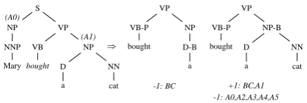
Figure 2: Examples of ASTmstructured features.
and automatic Charniak parse trees (Charniak, 2000) as provided for the CoNLL 2005 evaluation campaign (Carreras and M`arquez, 2005). SRL can be decomposed into two tasks: boundary detec-tion, where the word sequences that are arguments of a predicate wordware identified, and role clas-sification, where each argument is assigned the proper role. The former task requires a binary Boundary Classifier (BC), whereas the second in-volves a Role Multi-class Classifier (RM).
5.1.1 Setup
If the constituency parse tree t of a sentence s is available, we can look at all the pairs hp, nii, whereniis any node in the tree andpis the node dominating w, and decide whetherni is an argu-ment node or not, i.e. whether it exactly dominates all and only the words encoding any ofw’s argu-ments. The objects that we classify are subsets of the input parse tree that encompass bothpand
ni. Namely, we use the ASTm structure defined in (Moschitti et al., 2008), which is the minimal tree that covers all and only the words ofpandni. In the ASTm,pandniare marked so that they can be distinguished from the other nodes. An ASTm is regarded as a positive example for BC ifniis an argument node, otherwise it is considered a nega-tive example. Posinega-tive BC examples can be used to train an efficient RM: for each rolerwe can train a classifier whose positive examples are argument nodes whose label is exactly r, whereas negative examples are argument nodes labeledr′ 6=r. Two ASTms extracted from an example parse tree are shown in Figure 2: the first structure is a negative example for BC and is not part of the data set of RM, whereas the second is a positive instance for BC and A1.
(i.e. 5.7%).
For RM we considered all the argument nodes of any of the six PropBank core roles (i.e. A0, . . . , A5) from all the available training sections, i.e. 2 through 21, for a total of 179,091 train-ing instances. Similarly, we collected 5,928 test instances from the annotations of Section 24. Columns Tr+ and Te+ of Table 1 show the num-ber of positive training and test examples, respec-tively, for BC and the role classifiers.
For all the linearized classifiers, we used 50 splits for the FMI stage and we set the threshold valueL= 50kandmaxexp= 1during FMI and TFX. We did not validate these parameters, which we know to be sub-optimal. These values were selected during the development of the software because, on a very small test bed, they resulted in a responsive and accurate system.
We should point out that other experiments have shown that linearization is very robust with re-spect to parametrization: due to the huge num-ber and variety of fragments in the TK space, dif-ferent choices of the parameters result in differ-ent explicit spaces and more or less efficidiffer-ent solu-tions, but in most cases the final accuracy of the linearized classifiers is affected only marginally. For example, it could be expected that reducing the number of splits during KSL would improve the final accuracy of a linearized classifier, as the weights used for FMI would then converge to the global optimum. Instead, we have observed that increasing the number of splits does not necessar-ily decrease the accuracy of the linearized classi-fier.
The evaluation on the whole SRL task using the official CoNLL’05 evaluator was not carried out because producing complete annotations re-quires several steps (e.g. overlap resolution, OvA or Pairwise combination of individual role classi-fiers) that would shade off the actual impact of the methodology on classification.
5.1.2 Results
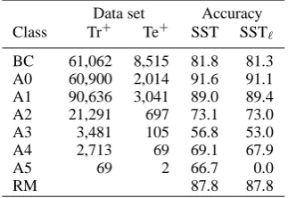
The left side of Table 1 shows the distribution of positive data points in the training and test sets of each classifier. Columns SST and SSTℓ compare side by side the F1 measure of the non-linearized and linearized classifier for each class. The accu-racy of the RM classifier is the percentage of cor-rect class assignments.
We can see that the accuracy of linearized clas-sifiers is always in line with vanilla SST, even
Data set Accuracy Class Tr+ Te+ SST SSTℓ
BC 61,062 8,515 81.8 81.3 A0 60,900 2,014 91.6 91.1 A1 90,636 3,041 89.0 89.4 A2 21,291 697 73.1 73.0 A3 3,481 105 56.8 53.0 A4 2,713 69 69.1 67.9
A5 69 2 66.7 0.0
[image:6.595.336.498.63.174.2]RM 87.8 87.8
Table 1: Number of positive training (Tr+) and test (Te+) examples in the SRL dataset. Accuracy of the non-linearized (SST) and linearized (SSTℓ) bi-nary classifiers (i.e. BC, A0, . . . A5) is F1measure. Accuracy of RM is the percentage of correct class assignments.
if the selected linearization parameters generate a very rough approximation of the original frag-ment space, generally consisting of billions of fragments. BCℓ (i.e. the linearized BC) has an F1of 81.3, just 0.5% less than BC, i.e. 81.8. Con-cerning RMℓ, its accuracy is the same as the non linearized classifier, i.e. 87.8.
We should consider that the linearization frame-work can drastically improve the efficiency of learning and classification when dealing with large amounts of data. For a linearized classifier, we consider training time to be the overall time re-quired to carry out the following activities: KSL, FMI, TFX on training data and ESL. Similarly, we consider test time the time necessary to per-form TFX on test data and ESC. Training BC took more than two days of CPU time and testing about 4 hours, while training and testing the linearized boundary classifier required only 381 and 25 min-utes, respectively. That is, on the same amount of data we can train a linearized classifier about 8 times as fast, and test it in about 1 tenth of the time. Concerning RM, sequential training of the 6 models took 2,596 minutes, while testing took 27 minutes. The linearized role multi classifier re-quired 448 and 24 minutes for training and test-ing, respectively, i.e. training is about 5 times as fast while testing time is about the same. If com-pared with the boundary classifier, the improve-ment in efficiency is less evident: indeed, the rel-atively small size of the role classifiers data sets limits the positive effect of splitting training data into smaller chunks.
struc-tures as input to our classifiers: nodes whose la-bel end with “-P” are predicate nodes, while nodes whose label ends with “-B” are candidate argu-ment nodes.
All the most relevant fragments encode the min-imum sub-tree encompassing the predicate and the argument node. This kind of structured feature subsumes several features traditionally employed for explicit SRL models: the Path (i.e. the se-quence of nodes connecting the predicate and the candidate argument node), Phrase Type (i.e. the label of the candidate argument node), Predicate POS (i.e. the POS of the predicate word), Posi-tion (i.e. whether the argument is to the left or to the right of the predicate) and Governing Category (i.e. the label of the common ancestor) defined in (Gildea and Jurafsky, 2002).
The linearized model for BC contains about 160 thousand fragments. Of these, about 70 and 33 thousand encompass the candidate argument or the predicate node, respectively. About 16 thousand fragments contain both.
5.2 Question Classification
For question classification we used the data set from the TREC 10 QA evaluation campaign2, con-sisting of 5,500 training and 500 test questions.
5.2.1 Setup
Given a question, the QC task consists in selecting the most appropriate expected answer type from a given set of possibilities. We adopted the question taxonomy known as coarse grained, which has been described in (Zhang and Lee, 2003) and (Li and Roth, 2006), consisting of six non overlap-ping classes: Abbreviations (ABBR), Descrip-tions (DESC, e.g. definiDescrip-tions or explanaDescrip-tions), En-tity (ENTY, e.g. animal, body or color), Human (HUM, e.g. group or individual), Location (LOC, e.g. cities or countries) and Numeric (NUM, e.g. amounts or dates).
For each question, we generate the full parse of the sentence and use it to train SST and (lin-earized) SSTℓ models. The automatic parses are obtained with the Stanford parser3 (Klein and Manning, 2003). We actually have only 5,483 sen-tences in our training set, due to parsing issues with a few of them.
2http://l2r.cs.uiuc.edu/cogcomp/Data/
QA/QC/
3http://nlp.stanford.edu/software/
lex-parser.shtml
Data set Accuracy Class Tr+ Te+ SST SSTℓ
[image:7.595.337.497.63.164.2]ABBR 89 9 80.0 87.5 DESC 1,164 138 96.0 94.5 ENTY 1,269 94 63.9 63.5 HUM 1,231 65 88.1 87.2 LOC 834 81 77.6 77.9 NUM 896 113 80.4 80.8 Overall 86.2 86.6
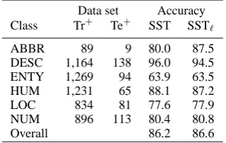
Table 2: Number of positive training (Tr+) and test (Te+) examples in the QA dataset. Accuracy of the non-linearized (SST) and linearized (SSTℓ) bi-nary classifiers is F1 measure. Overall accuracy is the percentage of correct class assignments.
The classifiers are arranged in a one-vs.-all (OvA) configuration, where each sentence is a positive example for one of the six classes, and negative for the other five. Given the very small size of the data set, we used S = 1during KSL for the linearized classifier (i.e. we didn’t parti-tion training data). We carried out no validaparti-tion of the parameters, and we used maxexp = 4 and
L = 50k in order to generate a rich fragment space.
5.2.2 Results
Table 2 shows the number of positive examples in the training and test set of each individual bi-nary classifiers. Columns SST and SSTℓcompare the F1measure of the vanilla and linearized classi-fiers on the individual classes, and the accuracy of the complete QC task (Row Overall) in terms of percentage of correct class assignments. Also in this case, we can notice that the accuracy of the linearized classifiers is always in line with non-linearized ones, e.g. 86.6 vs. 86.2 for the multi-classifiers. These results are lower than those de-rived in (Moschitti, 2006; Moschitti et al., 2007), i.e. 88.2 and 90.4, respectively, where the param-eters for each classifier were carefully optimized.
QC Fragment space. Tables from 4 to 9 list the top fragments identified for each class4.
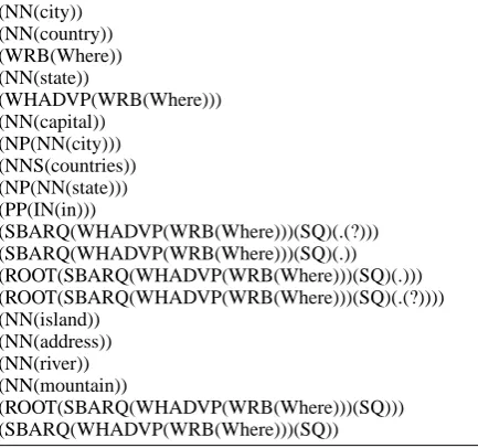
As expected, for all the categories the domain lexical information is very relevant. For example, film, color, book, novel and sport for ENTY or city, country, state and capital for LOC. Of the six classes, ENTY (Table 6) is mostly characterized by lexical features. Interestingly, function words, which would have been eliminated by a pure In-formation Retrieval approach (i.e. by means of
4Some categories show meaningful syntactic fragments
standard stop-list), are in the top positions, e.g.: why and how for DESC, what for ENTY, who for HUM, where for LOC and when for NUM. For the latter, also how seems to be important suggesting that features may strongly characterize more than one given class.
Characteristic syntactic features appear in the top positions for each class, for example: (VP (VB (stand)) (PP)), which suggests that stand should be followed by a prepositional phrase to character-ize ABBR; or (NP (NP (DT) (NN (abbreviation))) (PP)), which suggests that, to be in a relevant pat-tern, abbreviation should be preceded by an article and followed by a PP. Also, the syntactic struc-ture is useful to differentiate the use of the same important words, e.g. (SBARQ (WHADVP (WRB (How))) (SQ) (.)) for DESC better characterizes the use of how with respect to NUM, in which a relevant use is (WHADJP (WRB (How)) (JJ)).
In (Moschitti et al., 2007) it was shown that the use of TK improves QC of 1.2 percent points, i.e. from 90.6 to 91.8: further analysis of these frag-ments may help us to device compact, less sparse syntactic features and design more accurate mod-els for the task.
6 Discussion
The fact that our model doesn’t always improve the accuracy of a standard SST model might be related to the process of splitting training data and employing locally estimated weights during FMI.
Concerning the experiments presented in this paper, this objection might apply to the results on SRL, where we used 50 splits to identify the most relevant fragments, but not to those on QC, where given the limited size of the data set we decided not to split training data at all as explained in Sec-tion 5.2. Furthermore, as we already discussed, we have evidence that there is no direct correlation between the number of splits used for KSL and the accuracy of the resulting classifier. After all, the optimization carried out during ESL is global, and we can assume that, if we mined enough frag-ments during FMI, than those actually retained by the global linear model would be by and large the same, regardless of the split configuration.
More in general, feature selection may give an improvement to some learning algorithm but if it can help SVMs is debatable, since its related the-ory show that they are robust to irrelevant fea-tures. In our specific case, we remove features
(ADJP(RB-B)(VBN-P)) (NP(VBN-P)(NNS-B)) (S(NP-B)(VP))
[image:8.595.305.527.75.215.2](VP(VBD-P(said))(SBAR)) (VP(VB-P)(NP-B)) (NP(VBG-P)(NNS-B)) (VP(VBD-P)(NP-B)) (VP(VBG-P)(NP-B)) (VP(VBZ-P)(NP-B)) (VP(VBN-P)(NP-B)) (VP(VBP-P)(NP-B)) (NP(NP-B)(VP)) (NP(VBG-P)(NN-B)) (S(S(VP(VBG-P)))(NP-B))
Table 3: Best fragments for SRL BC.
(NN(abbreviation))
(NP(DT)(NN(abbreviation))) (NP(DT(the))(NN(abbreviation))) (IN(for))
(VB(stand)) (VBZ(does)) (PP(IN))
(VP(VB(stand))(PP))
(NP(NP(DT)(NN(abbreviation)))(PP)) (SQ(VBZ)(NP)(VP(VB(stand))(PP)))
(SBARQ(WHNP)(SQ(VBZ)(NP)(VP(VB(stand))(PP)))(.)) (SQ(VBZ(does))(NP)(VP(VB(stand))(PP)))
[image:8.595.307.527.414.581.2](VP(VBZ)(NP(NP(DT)(NN(abbreviation)))(PP)))
Table 4: Best fragments for the ABBR class.
(WRB(Why))
(WHADVP(WRB(Why))) (WHADVP(WRB(How))) (WHADVP(WRB)) (VB(mean)) (VBZ(causes)) (VB(do))
(ROOT(SBARQ(WHADVP(WRB(How)))(SQ)(.))) (ROOT(SBARQ(WHADVP(WRB(How)))(SQ)(.(?)))) (SBARQ(WHADVP(WRB(How)))(SQ))
(WRB(How))
(SBARQ(WHADVP(WRB(How)))(SQ)(.)) (SBARQ(WHADVP(WRB(How)))(SQ)(.(?))) (SBARQ(WHADVP(WRB(Why)))(SQ)) (ROOT(SBARQ(WHADVP(WRB(Why)))(SQ))) (SBARQ(WHADVP(WRB))(SQ))
Table 5: Best fragments for the DESC class.
(NN(film)) (NN(color)) (NN(book)) (NN(novel)) (NN(sport)) (WP(What)) (NN(fear)) (NN(movie)) (NN(word)) (VP(VBN(called))) (NN(game)) (NP(DT)(NN(fear))) (NP(NP(DT)(NN(fear)))(PP))
[image:8.595.308.527.613.747.2](NN(company)) (WP(Who)) (WHNP(WP(Who))) (NN(name)) (NN(team)) (NN(baseball)) (WHNP(WP)) (NN(character)) (NNP(President)) (NN(leader)) (NN(actor)) (NN(president)) (JJ(Whose)) (VP(VBD)(NP)) (NP(NP)(JJ)(NN(name))) (VP(VBD)(VP)) (NN(organization))
(VP(VBD)(NP)(PP(IN)(NP))) (SBARQ(WHNP(WP(Who)))(SQ)(.)) (ROOT(SBARQ(WHNP(WP(Who)))(SQ)(.))) (ROOT(SBARQ(WHNP(WP(Who)))(SQ)(.(?)))) (SBARQ(WHNP(WP(Who)))(SQ)(.(?)))
Table 7: Best fragments for the HUM class.
(NN(city)) (NN(country)) (WRB(Where)) (NN(state))
(WHADVP(WRB(Where))) (NN(capital))
(NP(NN(city))) (NNS(countries)) (NP(NN(state))) (PP(IN(in)))
(SBARQ(WHADVP(WRB(Where)))(SQ)(.(?))) (SBARQ(WHADVP(WRB(Where)))(SQ)(.)) (ROOT(SBARQ(WHADVP(WRB(Where)))(SQ)(.))) (ROOT(SBARQ(WHADVP(WRB(Where)))(SQ)(.(?)))) (NN(island))
(NN(address)) (NN(river)) (NN(mountain))
[image:9.595.73.290.335.538.2](ROOT(SBARQ(WHADVP(WRB(Where)))(SQ))) (SBARQ(WHADVP(WRB(Where)))(SQ))
Table 8: Best fragments for the LOC class.
(WRB(How))
(WHADVP(WRB(When))) (WRB(When))
(JJ(many)) (NN(year))
(WHADJP(WRB)(JJ)) (NP(NN(year)))
(WHADJP(WRB(How))(JJ)) (NN(date))
(SBARQ(WHADVP(WRB(When)))(SQ)(.(?))) (SBARQ(WHADVP(WRB(When)))(SQ)(.)) (NN(day))
(NN(population))
(ROOT(SBARQ(WHADVP(WRB(When)))(SQ)(.))) (ROOT(SBARQ(WHADVP(WRB(When)))(SQ)(.(?)))) (JJ(average))
(NN(number))
Table 9: Best fragments for the NUM class.
whose SVM weights are the lowest, i.e. those that are (almost) irrelevant for the SVM. There-fore, the chance of this resulting in an improve-ment is rather low.
With respect to cases where our model is less accurate than a standard SST, we should consider that our choice of parameters is sub-optimal and we adopt a very aggressive feature selection strat-egy, that only retains a few thousand features from a space where there are hundreds of millions of different features.
7 Conclusions
We introduced a novel framework for support vec-tor classification that combines advantages of con-volution kernels, i.e. the generation of a very high dimensional structure space, with the efficiency and clarity of explicit representations in a linear space.
For this paper, we focused on the SubSet Tree kernel and verified the potential of the proposed solution on two NLP tasks, i.e. semantic role labeling and question classification. The exper-iments show that our framework drastically re-duces processing time, e.g. boundary classifica-tion for SRL, while preserving the accuracy.
We presented a selection of the most relevant fragments identified for the SRL boundary classi-fier as well as for each class of the coarse grained QC task. Our analysis shows that our frame-work can discover state-of-the-art features, e.g. the Path feature for SRL. We believe that shar-ing these fragments with the NLP community and studying them in more depth will be useful to identify new, relevant features for the character-ization of several learning problems. For this purpose, we made available the fragment spaces athttp://danielepighin.netand we will keep
them updated with new set of experiments on new tasks, e.g. SRL based on FrameNet and VerbNet, e.g. (Giuglea and Moschitti, 2004).
References
Fabio Aiolli, Giovanni Da San Martino, Alessandro Sper-duti, and Alessandro Moschitti. 2006. Fast on-line kernel learning for trees. In Proceedings of ICDM’06.
Stephan Bloehdorn and Alessandro Moschitti. 2007a. Com-bined syntactic and semantic kernels for text classification. In Proceedings of ECIR 2007, Rome, Italy.
Stephan Bloehdorn and Alessandro Moschitti. 2007b. Struc-ture and semantics for expressive text kernels. In In Pro-ceedings of CIKM ’07.
Nicola Cancedda, Eric Gaussier, Cyril Goutte, and Jean Michel Renders. 2003. Word sequence kernels. Journal of Machine Learning Research, 3:1059–1082.
Xavier Carreras and Llu´ıs M`arquez. 2005. Introduction to the CoNLL-2005 Shared Task: Semantic Role Labeling. In Proceedings of CoNLL’05.
Eugene Charniak. 2000. A maximum-entropy-inspired parser. In Proceedings of NAACL’00.
Michael Collins and Nigel Duffy. 2002. New Ranking Al-gorithms for Parsing and Tagging: Kernels over Discrete Structures, and the Voted Perceptron. In Proceedings of ACL’02.
Aron Culotta and Jeffrey Sorensen. 2004. Dependency Tree Kernels for Relation Extraction. In Proceedings of ACL’04.
Chad Cumby and Dan Roth. 2003. Kernel Methods for Re-lational Learning. In Proceedings of ICML 2003.
Mona Diab, Alessandro Moschitti, and Daniele Pighin. 2008. Semantic role labeling systems for Arabic using kernel methods. In Proceedings of ACL-08: HLT, pages 798– 806.
Daniel Gildea and Daniel Jurafsky. 2002. Automatic label-ing of semantic roles. Computational Llabel-inguistics, 28:245– 288.
Ana-Maria Giuglea and Alessandro Moschitti. 2004. Knowledge discovery using framenet, verbnet and prop-bank. In A. Meyers, editor, Workshop on Ontology and Knowledge Discovering at ECML 2004, Pisa, Italy.
Alfio Gliozzo, Claudio Giuliano, and Carlo Strapparava. 2005. Domain kernels for word sense disambiguation. In Proceedings of ACL’05, pages 403–410.
Hans P. Graf, Eric Cosatto, Leon Bottou, Igor Durdanovic, and Vladimir Vapnik. 2004. Parallel support vector ma-chines: The cascade svm. In Neural Information Process-ing Systems.
Isabelle Guyon and Andr´e Elisseeff. 2003. An introduc-tion to variable and feature selecintroduc-tion. Journal of Machine Learning Research, 3:1157–1182.
David Haussler. 1999. Convolution kernels on discrete struc-tures. Technical report, Dept. of Computer Science, Uni-versity of California at Santa Cruz.
T. Joachims. 2000. Estimating the generalization perfor-mance of a SVM efficiently. In Proceedings of ICML’00.
Hisashi Kashima and Teruo Koyanagi. 2002. Kernels for semi-structured data. In Proceedings of ICML’02.
Jun’ichi Kazama and Kentaro Torisawa. 2005. Speeding up training with tree kernels for node relation labeling. In Proceedings of HLT-EMNLP’05.
Dan Klein and Christopher D. Manning. 2003. Accurate unlexicalized parsing. In Proceedings of ACL’03, pages 423–430.
Taku Kudo and Yuji Matsumoto. 2003. Fast methods for kernel-based text analysis. In Proceedings of ACL’03. Taku Kudo, Jun Suzuki, and Hideki Isozaki. 2005.
Boosting-based parse reranking with subtree features. In Proceed-ings of ACL’05.
Xin Li and Dan Roth. 2006. Learning question classifiers: the role of semantic information. Natural Language En-gineering, 12(3):229–249.
Alessandro Moschitti and Fabio Massimo Zanzotto. 2007. Fast and effective kernels for relational learning from texts. In ICML’07.
Alessandro Moschitti, Silvia Quarteroni, Roberto Basili, and Suresh Manandhar. 2007. Exploiting syntactic and shal-low semantic kernels for question/answer classification. In Proceedings of ACL’07.
Alessandro Moschitti, Daniele Pighin, and Roberto Basili. 2008. Tree kernels for semantic role labeling. Compu-tational Linguistics, 34(2):193–224.
Alessandro Moschitti. 2006. Efficient convolution kernels for dependency and constituent syntactic trees. In Pro-ceedings of ECML’06, pages 318–329.
Julia Neumann, Christoph Schnorr, and Gabriele Steidl. 2005. Combined SVM-Based Feature Selection and Clas-sification. Machine Learning, 61(1-3):129–150.
Martha Palmer, Daniel Gildea, and Paul Kingsbury. 2005. The proposition bank: An annotated corpus of semantic roles. Comput. Linguist., 31(1):71–106.
J. Pei, J. Han, Mortazavi B. Asl, H. Pinto, Q. Chen, U. Dayal, and M. C. Hsu. 2001. PrefixSpan Mining Sequential Pat-terns Efficiently by Prefix Projected Pattern Growth. In Proceedings of ICDE’01.
Daniele Pighin and Alessandro Moschitti. 2009. Efficient linearization of tree kernel functions. In Proceedings of CoNLL’09.
Alain Rakotomamonjy. 2003. Variable selection using SVM based criteria. Journal of Machine Learning Research, 3:1357–1370.
Libin Shen, Anoop Sarkar, and Aravind k. Joshi. 2003. Us-ing LTAG Based Features in Parse RerankUs-ing. In Proceed-ings of EMNLP’06.
Jun Suzuki and Hideki Isozaki. 2005. Sequence and Tree Kernels with Statistical Feature Mining. In Proceedings of NIPS’05.
Kristina Toutanova, Penka Markova, and Christopher Man-ning. 2004. The Leaf Path Projection View of Parse Trees: Exploring String Kernels for HPSG Parse Selec-tion. In Proceedings of EMNLP 2004.
Vladimir N. Vapnik. 1998. Statistical Learning Theory. Wiley-Interscience.
Ellen M. Voorhees. 2001. Overview of the trec 2001 ques-tion answering track. In In Proceedings of the Tenth Text REtrieval Conference (TREC, pages 42–51.
Jason Weston, Sayan Mukherjee, Olivier Chapelle, Massimil-iano Pontil, Tomaso Poggio, and Vladimir Vapnik. 2001. Feature Selection for SVMs. In Proceedings of NIPS’01.
Jason Weston, Andr´e Elisseeff, Bernhard Sch¨olkopf, and Mike Tipping. 2003. Use of the zero norm with lin-ear models and kernel methods. J. Mach. Llin-earn. Res., 3:1439–1461.