Modeling heaped duration data : an application to neonatal mortality

warwick.ac.uk/lib-publications

Arulampalam, Wiji, Corradi, Valentina and Gutknecht, Daniel (2017) Modelling heaped duration data : an application to neonatal mortality. Journal of Econometrics, 200 (2). pp. 363-377. doi:10.1016/j.jeconom.2017.06.016

Permanent WRAP URL:

http://wrap.warwick.ac.uk/82248

Copyright and reuse:

The Warwick Research Archive Portal (WRAP) makes this work by researchers of the University of Warwick available open access under the following conditions. Copyright © and all moral rights to the version of the paper presented here belong to the individual author(s) and/or other copyright owners. To the extent reasonable and practicable the material made available in WRAP has been checked for eligibility before being made available.

Copies of full items can be used for personal research or study, educational, or not-for-profit purposes without prior permission or charge. Provided that the authors, title and full bibliographic details are credited, a hyperlink and/or URL is given for the original metadata page and the content is not changed in any way.

Publisher’s statement:

© 2018, Elsevier. Licensed under the Creative Commons Attribution-NonCommercial-NoDerivatives 4.0 International http://creativecommons.org/licenses/by-nc-nd/4.0/

A note on versions:

The version presented here may differ from the published version or, version of record, if you wish to cite this item you are advised to consult the publisher’s version. Please see the ‘permanent WRAP URL’ above for details on accessing the published version and note that access may require a subscription.

Modeling Heaped Duration Data: An Application to Neonatal

Mortality

Wiji Arulampalam†

Warwick University

Valentina Corradi ‡

Surrey University

Daniel Gutknecht§

Mannheim University

April 12, 2016

Abstract

In 2005, the Indian Government launched a conditional cash-incentive program to en-courage institutional delivery. This paper studies the effects of the program on neonatal mortality using district-level household survey data. We model mortality using survival analysis, paying special attention to substantial heaping, a form of measurement error, present in the data. The main objective of this paper is to provide a set of sufficient con-ditions for identification and consistent estimation of the (discretized) baseline hazard accounting for heaping and unobserved heterogeneity. Our identification strategy re-quires neither administrative data nor multiple measurements, but a correctly reported duration point and the presence of some flat segment(s) in the baseline hazard. We es-tablish the asymptotic properties of the maximum likelihood estimator and derive a set of specification tests that allow, among other things, to test for the presence of heaping and to compare different heaping mechanisms. Our empirical findings do not suggest a significant reduction of mortality in treated districts. However, they do indicate that accounting for heaping matters for the estimation of the hazard parameters.

Keywords:Discrete Time Duration Model, Heaping, Measurement Error, Parameters on the Boundary, Neonatal Mortality.

JEL Classification: C12, C21, C24, C41.

∗

We are grateful to the editors Tom Wansbeek and Yingyao Hu and two anonymous referees as well as Aureo de Paula, Giovanni Forchini, Federico Martellosio, and Mervin Silvapulle for many useful comments and suggestions that helped to greatly improve the paper. We would also like to thank Marco Alfano and Artemisa Flores for help with the data preparation. Comments received from seminar participants at Oxford University, the 6th Italian Conference on Econometrics and Empirical Economics (ICEEE) in Salerno, Groningen University, CEMFI, ENSAI, Mannheim University, Munich University, and Leicester University are gratefully acknowledged.

†

Department of Economics, University of Warwick, Coventry CV4 7AL, UK. Tel. +44(0)2476 523471; email: [email protected]

‡

Department of Economics, University of Surrey, School of Economics, Guildford GU2 7XH, UK, Tel. +44(0)1483 693914; email: [email protected]

§

1

Introduction

India has one of the largest neonatal mortality and maternal mortality rates in the world.1 Around 32 neonates per 1000 live births (around 876,200 children) die within the first month of life each year (Roy et al., 2013; Save the Children, 2013) and among these babies, 309,000 die on the first day. Moreover, around 200 mothers die during pregnancy and child birth per 100,000 live births each year. In order to tackle this huge problem, the Indian Government introduced a conditional cash-incentive (Janani Suraksha Yojana- JSY) program in 2005 to encourage institutional delivery. The Indian Government also deployed volunteer Accredited Social Health Activists to help mothers with antenatal and postnatal care during the crucial pre and post birth period.

This paper studies the effects of the above Indian cash-incentive program on neonatal mortality using district-level household survey data. We focus on the neonatal period, since the effects of the program are expected to be most pronounced soon after birth when postnatal care is provided. We model mortality using survival analysis, paying special attention to a characteristic of the reported duration data, which is apparent heaping at 5,10,15, . . . days (durations which are multiple of five days). These heaping effects in the data are likely to be due to measurement error and lead, if neglected, to inconsistency in the estimation of the underlying hazard function (e.g., Torelli and Trivellato, 1993, and Wolff and Augustin, 2003).

In addressing heaping effects due to misreporting, this paper makes several method-ological contributions in the modeling of discrete time duration data when the data is characterized by abnormal concentrations at certain duration points. First, we provide a set of sufficient conditions for the pointwise identification and consistent estimation of the (discretized) baseline hazard and other parameters of a proportional hazard model account-ing for heapaccount-ing and unobserved heterogeneity. We pay particular attention to the baseline hazard to gauge the effect of the policy that was specifically intended to reduce neonatal mortality. Second, we derive various specification tests to test (i) for the presence as well as (ii) for different patterns of heaping effects in our model, and (iii) to assess the effects of policy changes on the baseline hazard.2 These tests provide the applied researcher with a set of tools that enable her to verify the validity of different model specifications.

Despite the prevalence of heaping in survey data, the econometric literature on identifi-cation and estimation of duration models under heaping is rather limited. In the presence of misreported durations, Abrevaya and Hausman (1999) derive a set of sufficient conditions under which the monotone rank estimator remains a consistent estimator for the covari-ate parameters of an accelercovari-ated failure time and proportional hazard model. Torelli and Trivellato (1993) and Augustin and Wolff (2004) derive procedures that allow for different forms of heaping, but assume a parametric specification for the hazard function, which is not suitable if the ultimate goal of an analysis is inference on a policy change that might not have affected the entire hazard function. Petoussis, Gill and Zeelenberg (1997) treat heaped durations as missing values and use the Expectation-Maximization (EM) algorithm

1_{The neonatal period is defined as the first 28 days after birth.} 2

to estimate a proportional hazard model. Finally, Heitjan and Rubin (1990) suggest an EM-based multiple imputation method for inference in the presence of heaped data. The authors do, however, not cover the duration case. Moreover, note that none of the above papers deals with identification of the baseline hazard function.

Another paper related to ours is Ham, Li and Shore-Sheppard (2014): studying the em-ployment dynamics of single mothers in the Survey of Income and Program Participation (SIPP), the authors establish identification of a (discretized) baseline hazard function in a duration model with multiple spells in the presence of seam bias and unobserved hetero-geneity.3 An appealing aspect of their identification strategy is that it can be applied to samples that consist not only of newly sampled (“fresh”), but also of left-censored spells, a common feature of labor market history survey data.4 The key difference between the identification strategy of Ham, Li and Shore-Sheppard (2014) and ours is that they require at least two measurements of the same duration (collected from different survey waves), where only one is affected by seam bias. Since we do not have multiple measurements at disposal in our data, their methodology cannot be applied in our context.

The identification strategy of our paper is based on a set of minimal assumptions on the shape of the discretized hazard function. That is, neither do we require administrative data nor do we make assumptions about the validity of observations closer to the interview date.5 Instead, our identification strategy requires, as key ingredients, the existence of at least one correctly reported duration point and the presence of some flat segment(s) in the baseline hazard, which includes this correctly reported duration point. The length of the flat segment(s) required depends on the complexity of the heaping process.

Heuristically speaking, the constant part of the baseline hazard enables us to identify the parameters of the heaping process, i.e. the probability of rounding to a heaped value, and hence the rest of the baseline hazard parameters. Information about the correctly reported duration and the flat segment can stem from different sources and does not have to come from a specific data set. For instance, in our empirical example we partially rely on information from a verbal autopsy report on neonatal mortality in Uttar Pradesh, the most populated Indian state, which suggests that assuming a flat hazard segment towards 18 days is a relatively plausible assumption. The likelihood function is then constructed down-weighting the contribution of heaped durations and over-weighting the contribution of non heaped durations. This adjustment ensures consistent estimation of both heaping and baseline hazard parameters in the case of a parametric specification of the unobserved heterogeneity component.6

3_{Seam bias, another common form of measurement error in multi-wave survey data, is characterized by}

an over-reported frequency of spell failures at the seam of different survey waves.

4_{In particular, the authors show that identification from left-censored spells can be obtained without}

restricting duration dependence by imposing that misreporting parameters are identical for left-censored and for newly begun spells.

5

In fact, we are unable to use durations sampled closer to the interview date as a ‘validation sample’ of ‘correctly’ reported observations as these durations exhibit similar heaping patterns as the ones that lie further away from the interview date. This suggests that heaping in our data is not mainly driven by recall error.

6_{We rely on a parametric specification for the unobserved heterogeneity distribution to obtain a closed}

Moreover, in the supplementary material of the paper we provide an informal discussion on how our methodology can be extended to identify the parameters of different discrete duration models (e.g., Han and Hausman, 1990; Sueyoshi, 1995) as well as of standard ordered choice models. Since ordered choice models are also used in the analysis of count data such as number of doctor visits or cigarette consumption, where heaping is often a feature of the data, we deem this an important extension of our theoretical identification results.

Finally, we derive a number of specification tests that allow applied researchers to check the validity of different heaping mechanisms as well as model specifications. The tests are based on the likelihood ratio statistic and can be straightforwardly computed. However, when some of the heaping parameters lie on the boundary of the parameter space, the limiting distribution of the statistic under the null hypothesis follows a mixture of standard χ2-distributions, and critical values can be difficult to construct. Thus, we establish the first order validity of critical values based on the ‘M out of N’ bootstrap.

The rest of this paper is organized as follows. Section 2 describes the setup and the heaping model we consider. As a main result, we provide a set of sufficient conditions for the identification of the parameters of a discrete time duration model. Section 3 derives the likelihood function and establishes the asymptotic properties of the maximum likelihood estimator. Since we do not impose a strictly positive probability of rounding, we account for the possibility of parameters on the boundary of the parameter space (Andrews, 1999). Section 4 outlines how to conduct inference in our context. More specifically, the paper proposes two specification tests to detect whether heaping matters in a statistical sense and, if it matters, to determine whether any of the heaping parameters lie on the boundary. Section 5 then extends the setup of Sections 3 and 4 to analyze the effects of potential policy changes on duration outcomes when inference is hampered by a change in the reporting behavior over time.7 That is, we discuss the possibility that treatment not only affects the parameters of interest, but also the reporting behavior (and thus the pattern of heaping). We also develop various specification tests to verify these conjectures statistically. Finally, Section 6 contains the empirical example and reports our findings. First, a specification test and model estimates indicate that heaping plays an important role in our data. Second, we do not find evidence for an increase in survival probability of babies born in districts that were treated. However, since our analysis was conducted using only babies born in districts that were eventually treated, it remains to be established whether the actual treatment effect exhibits a similar pattern, too. Section 7 concludes. Figures, graphs, and tables can be found in Appendix I, while Appendix II contains the proofs of our main technical results (Proposition 1 and Theorem 2). All proofs of Sections 4 and 5, some additional specification tests (together with their proofs), instructions on how to implement the bootstrap procedure as well as other supporting material have been collected in the supplementary material.

As a final remark on notation, note that lower case letters are employed throughout the paper to denote random variables as well as their realizations. Also, let K = dim(x) denote the dimension of any K×1 vector x with K ≥ 1, and define R = (−∞,∞) and R+= (0,∞).

for recent advances in dealing with unobserved heterogeneity in duration models with correctly reported observations.

7

2

Identification

We begin by outlining our setup. Assuming a Mixed Proportional Hazard (MPH) model for the unobservable true durations, our objective is to recover the underlying model parameters from the observable and potentially mismeasured durations.

Letτ_i∗be a continuous, non-negative random variable denoting the (continuous) duration time of individual i. The associated hazard function at time τ∗ is given by:

λi(τ∗) = lim

∆→0Pr(τ

∗

i < τ

∗

+ ∆|τ_i∗>τ∗)/∆.

We parameterize this hazard as:

λi(τ∗|zi, ui) =λ0(τ∗) exp(zi0β+ui),

whereλ0(τ∗) is the baseline hazard,ui is the individual unobserved heterogeneity, andzi a

set of time invariant covariates. In most empirical studies, however, time is observed on a discrete scale, e.g., in days in the illustration of Section 6. Thus, in the following, we will assume that a continuous durationτ_i∗∈[τ, τ+1) is recorded asτ, whereτ denotes a discrete time period, so that the sample of (discrete) durations is given by τi fori= 1, . . . , N. The discrete time hazard for our model can then be written as:

hi(τ|zi, ui) = Pr [τi∗< τ + 1|τi∗ >τ, zi, ui]

=1−exp

−

Z τ+1

τ

λi(s|zi, ui)ds

(1)

=1−exp

−exp

z_i0β+γ(τ)

+ui

,

where γ(τ) = lnR_ττ+1λ0(s)ds. Due to misreporting, however, the researcher does not

ob-serveτi directly, butti, a potentially mismeasured version of it.

More specifically, the form of misreporting we address in this paper is referred to as “heaping” in the literature and describes the phenomenon of observing an over- and under-reporting of failures at certain time periods. Formally, assume that excessive concentrations of reported failures occur at time period h∗ and at multiplesj·h∗ with j= 0,1, . . . , j and j a finite, non-negative integer denoting the maximum number of heaps in the data.8 _For

instance, in the example of the 28 day neonatal mortality period, if reported exits are heaped at values that are multiples of 5 periods and the last heap occurs at period 25, then h∗ = 5 and j = 1,2,3,4,5. A stylized version of this case has been illustrated in Figure 1 of Appendix I.

Next, to identify the baseline hazard from possibly misreported observations, we impose a structure on the heaping process: letr denote the maximum number of time periods that a duration can be rounded to, e.g. with heaps at 5 and 10 days in the stylized example above, r is set equal to 2 so that two periods to the right and to the left of each heap point are associated with that heap.

8_{Note that the equal distance between the heap points is a notational simplification, which could}

Furthermore, assume that all durationsτi,i∈1, . . . , N, fall into the setD={0,1, . . . , τ− 1}, where τ is some finite, positive integer and (τ −1) represents the maximum observed time period. We assume that all heaping is to observed duration points only.9 Then, denote the set of

(i) heaping points as:

DH=τ :τ =jh∗, j = 1,2, ..., j, jh∗< τ ; (ii) points that may be rounded up as:

DH−l_{=τ :τ =jh}∗_{−l, j= 1,2, ..., j, jh}∗_{−l < τ ;}

and (iii) points that may be rounded down as:

DH+l_{=τ :τ =jh}∗_{+l, j = 1,2, ..., j, jh}∗_{+l < τ ;}

for l = 1, ..., r. See Figure 2 in Appendix I for an illustration of the case where h∗ = 5, j= 2, andr = 2.

Moreover, assume that whenever the true duration τi falls onto one of the heaping points, it will be correctly reported. That is, for eachτi ∈ DH, ti =τia.s..10 However, when τi ∈ ∪r

l=1D

H−l_{∪ ∪}r

l=1D

H+l_{, it is either correctly reported or rounded (up or down) to the}

closest heaping point belonging toDH. Thus, forl∈ {1, . . . , r}, let Pr (ti =τi+l) =pl and Pr (ti=τi) = 1−pl if τi ∈ DH−l. Analogously, let Pr (ti =τi−l) = ql and Pr (ti =τi) = 1−ql ifτi ∈ DH+l_{. In the example from above, a possible mechanism is for instance that}

a reported duration of say 10 days includes true durations of 11 and 12 (8 and 9), which have been rounded up (down) to 10 days (see again Figure 2 in Appendix I). The ps and theqs give the probabilities of these roundings.

Next, we outline our key identification assumption: Assumption H

(i) ∪r l=1D

H−l_{∩ ∪}r

l=1D

H+l_=∅;

(ii) For alll∈ {1, . . . , r},pl∈[0,1) and ql ∈[0,1);

(iii) There exists a j∈ {1, . . . , j} and ak < j·h∗−r such thatγ(k) =γ fork≤k≤j·h∗ and γ(k) =γ forj·h∗< k≤j·h∗+r;

(iv)ti =k if and only ifτi=k a.s..

Assumptions H(i)-(iv) are crucial for the identification of the baseline parameters and our identification result in Proposition 1 below. More specifically, H(i)-(ii) imply that duration points are only associated with one (the nearest) heaping point. In our example, this rules out that true durations of 7 days are, for instance, rounded to 5and 10 days simultaneously. We note, however, that our setup could also accommodate more complex heaping mech-anisms provided that the constant segment of the hazard required by H(iii) is sufficiently

9

For reasons of clarity, we will introduce censoring only in the next section.

10_{Note that the assumption that true durationsτi, which fall onto a heap point, are correctly observed}

large (see below). Moreover, in Section S2 of the supplementary material, we discuss a specification test that allows to discriminate between different (identified) heaping mech-anisms. Assumption H(ii) also imposes that durations belonging to either DH−l _{or D}H+l

withl= 1, . . . , rhave a strictly positive probability to be truthfully reported and to be ob-served. This assumption, which is essential to identify the parametersγ(k) for 1< k < τ, is deemed to be a rather mild regularity condition satisfied by most empirical settings. H(iii) requires that the baseline hazard is constant after time period k, but possibly at different levels on either side of the heaping pointj·h∗, which could for instance apply when heaping is asymmetric. Moreover, in H(iv), it is assumed thatkis observed without error. That is, k∈ DT, where DT is the set of truthfully reported durations and defined as the following complement set:

DT = ∪r_l=1DH−l_{∪ ∪}r

l=1D

H+l_{∪ D}Hc_.

Note that the set DT _{may not only containk, but also other duration points τ < τ, which}

are known to be correctly observed and do not lie in the union of∪r l=1D

H−l_,∪r

l=1D

H+l_{, and}

DH. Finally, we emphasize again that Assumptions H(iii)-(iv) are stronger than required as it would in principle suffice for the hazard to be constant over separate regions, not necessarily adjacent to each other, as long as these regions cover DH, DH−l_{, and D}H+l_,

l= 1, . . . , r.11

Heuristically, the assumption that the hazard is constant over a set of time periods, which includes (at least) a known true value, enables us to uniquely identify the γ parameter of the correctly reported time period as well as the parameters modeling the heaping process, i.e. thep’s and theq’s, in this region. Subsequently, we can use these identified probability parameters to pin down the rest of the baseline hazard parameters.

Before stating our main identification result, we need to define some more notation, which will be used in the following. Let θ ={β0, γ0}0 _{with γ = {γ(0), γ(1), . . . , γ(τ −1)}}0

and define the probability of survival at least until time period τ < τ in the absence of misreporting as:

Si(τ|zi, ui, θ) = Pr (τi≥τ|zi, ui, θ)

= τ−1

Y

s=0

exp −exp z0_iβ+γ(s) +ui

= τ−1

Y

s=0

exp −viexp z0iβ+γ(s)

,

11

wherevi ≡exp(ui). The probability for an exit event in τi < τ is: fi(τ|zi, ui, θ) = Pr (τi=τ|zi, ui, θ)

=Si(τ|zi, ui, θ)−Si(τ + 1|zi, ui, θ)

= τ−1

Y

s=0

exp −viexp z0_iβ+γ(s) (2)

−

τ

Y

s=0

exp −viexp z0iβ+γ(s)

.

Here, fi(τ|zi, ui, θ) denotes the probability of a duration equal to τ when there is no mis-reporting. However, because of the rounding, heaped values are over-reported while non-heaped values are under-reported, and this needs to be taken into account when constructing the likelihood function (see next section). Hereafter, let

φi(t|zi, vi, θ) = Pr (ti=t|zi, vi, θ)

withti denoting the discretereported duration. It is immediate to see the following for the four cases:

(I) forti ∈ DT, φi(t|zi, vi, θ) =fi(t|zi, vi, θ) ;

(II) forti ∈ DH−l, φi(t|zi, vi, θ) = (1−pl)fi(t|zi, vi, θ); (III) for ti∈ DH+l_{, φi(t|zi, vi, θ) = (1−ql)fi(t|zi, vi, θ);}

(IV) and forti ∈ DH,

φi(t|zi, vi, θ) = r

X

l=1

plfi(t−l|zi, vi, θ) + r

X

l=1

qlfi(t+l|zi, vi, θ) +fi(t|zi, vi, θ).

In summary, there are four different probabilities of exit events depending on whether the reported durationti is inDT,DH−l_,DH+l_{, orD}H_{respectively. Next, in order to obtain the}

unconditional versions of these probabilities, we introduce the following assumption on the unobserved heterogeneity distribution:

Assumption U:

(i) vi is identically and independently distributed;

(ii) The density ofv is gamma with unit mean and varianceσ−1; (iii) vi is independent of zi.

and findings by Han and Hausman (1990) as well as Meyer (1990) suggest that estimation results for discrete-time proportional hazard models where the baseline is left unspecified (as in our model) display little sensitivity to alternative distributional assumptions on vi.

Finally, we impose the following assumption on the observed heterogeneity distribution: Assumption Z: The support of at least one element z1i of zi, say Sz1, contains at least

two values and the corresponding element of β is non-zero. Moreover, the full support of zi,Sz, contains the zero vector.

Assumption Z is standard in the literature on identification of MPH models (cf. Elbers and Ridder, 1982; Ridder and Woutersen, 2003) and requires a minimum amount of variation in the covariates zi to identify β.

Using assumption U, the unconditional probabilities in case (I) above are given by:

Z

φi(t|zi, v, θ)g(v;σ)dv =

Z

Pr (τi =t|zi, v, θ)g(v;σ)dv

=

Z

Si(t|zi, v, θ)g(v;σ)dv−

Z

Si(t+ 1|zi, v, θ)g(v;σ)dv

= 1 +σ t−1

X

s=0

exp z_i0β+γ(s)

!!−σ−1

− 1 +σ t

X

s=0

exp z0_iβ+γ(s)

!!−σ−1

where the last equality uses the fact that there is a closed form expression under U(ii) (e.g., see Meyer (1990, p. 770)). Moreover, since the integral is a linear operator the probabilities for the cases (II) to (IV) can be derived accordingly. Then, we obtain the following identification result:

Proposition 1: Given AssumptionsZ, H,and U,we can uniquely identify{γ(0), . . . , γ(τ−

1), β0, σ}0together with the heaping probabilitiespl andql forl={1, . . . , r}from the reported durations.

The proof is provided in Appendix II and its heuristics are explained in the first of the following two remarks:

Remark 2.1: The proof of Proposition 1 is based on establishing a one to one relationship between exit probabilities and the baseline hazard (and the other model) parameters. Given Assumptions U, H(iii)-(iv) and an argument from Heckman and Singer (1984), we uniquely identify Pk

s=0exp(γ(s)) and so γ(k).Given this, and exploiting the flatness of the hazard,

as stated in H(iii), we identify the heaping probabilities ps and qs. Finally, using H(i), we sequentially identify all remainingγ parameters.12

Remark 2.2: In Section S3 of the supplementary material we show that the identification idea of Proposition 1 can also be applied or modified to apply to other discrete duration (e.g., Han and Hausman, 1990; Sueyoshi, 1995) and to standard ordered choice models, thus amplifying the applicability of Proposition 1 and the remaining results of the paper.

12_{Note that, similar to Assumption H, it appears from the proof in the Appendix that Assumption U is}

3

Estimation

Our next goal is to obtain consistent estimators forθ={θ0, σ, p1, . . . , pr, q1, . . . , qr}0from the

possibly misreported durations. Before setting up the likelihood function drawing from the derivations of the previous section for truthfully and misreported durations, we introduce censoring into our setup:

Assumption C:

(i) Durations are censored at a fixed time τ > jh∗ +r and the censoring mechanism is independent of the durations (type I censoring; Cox and Oakes, 1984);

(ii) Censoring is independent of the heaping process.

We note that C(i), which has been made in view of the illustration in Section 6, could be straightforwardly generalized to allow for varying censoring times across individuals (random censoring) as long as C(ii) remains satisfied.13 Furthermore, under Assumption C, the identification result established in Proposition 1 carries through to the censored case by defining a setDC _{for observations censored at τ, which does not overlap withD}H+l_,l=r.

Next, let δi be an indicator equal to one if the observation does not lie in DC and zero otherwise. Then, given Assumptions U, Z, and C and the definition of φi(·) from cases (I) to (IV) in Section 2, let the likelihood function be:

LN(θ) = N

Y

i=1

Z _n

φi(t|zi, v)δiSi(t|zi, v)(1−δi)

o

g(v;σ)dv

and so

lN(θ) = lnLN(θ) = N

X

i=1

ln

Z _n

φi(t|zi, v)δi_{Si(t|zi, v)}(1−δi) o

g(v;σ)dv.

Given the definition of φi(t|zi, v) and cases (I) through (IV) in Section 2, it is clear that the (log) likelihood function down-weights the contribution of heaped durations and over-weights the contribution of non heaped durations. Thus

b

θN = arg max θ∈ΘlN(θ)

θ†= arg max

θ∈Θ E (lN(θ)),

where Θ ⊂ RKβ+Kγ _×

R+×[0,1)2r denotes the parameter space with Kβ = dim(β) and

Kγ= dim(γ). Assumption D:

(i) (τi, x0i)0, i = 1, . . . , N, are i.i.d. random variables that take values in a subset of the product spaceR+×RKx.

(ii)E[τi4]<∞.

(iii) For all d= 1, ..., τ −1, _N1 P

i

1{τi =d} p

→Pr[τi =d]>0.

13

That is, a similar structure to cases (I) to (IV) in Section 2 could be used to determine the survival probabilities of censored spells (and thus their contribution to the likelihood). Also note that τ does not necessarily have to be greater thanτ > jh∗+ras long as it does not belong toDH

Together with Assumption H(ii), Assumption D(iii) ensures that asymptotically we observe exits in each time period untilτ−1, which in turn allows to estimate the associated baseline hazard parameters consistently.14 We now establish the asymptotic properties of θNb .

Theorem 2: Let Assumptions H,Z,U,Cand Dhold. Then: (i)

b

θN−θ†=op(1)

(ii)

√

N

b

θN −θ†

_d

→ inf ψ∈Ψ

(ψ−G)0I†(ψ−G)

,

with I† =E −∇2

θθlN(θ)/N

|_θ=θ†

,G∼N 0,I†−1

, and Ψ being a cone in RKβ+Kγ × R+×[0,1)2r.15

(iii) Let π†=

p†₁, ..., p†_r, q₁†, ..., q†_r

0

, if π†∈(0,1)2r,then √

Nθb_N −θ†

_d

→N0,I†−1_.

Theorem 2 establishes consistency of ˆθN in part (i) and its limiting distribution in parts (ii) and (iii). Its proof can be found in Appendix II. Note that the limiting distribution of the estimator depends on whether some heaping probability parameters lie on the boundary of the parameter space or not. That is, if one or more of the “true” probability parameters are equal to zero, the limiting distribution of √Nθb_N −θ†

is no longer normal as the information matrixI†−1 _{is not block diagonal in general, but takes the form in part (ii) (cf.}

Andrews, 1999).

4

Inference

Inference hinges on the limiting distribution of√N

b

θN−θ†

. However, as outlined above, if some of the heaping probability parameters lie on the boundary of the parameter space and the asymptotic distribution of √N

b

θN −θ†

is no longer normal, inference on the baseline hazard and other model parameters becomes more complicated. A solution in this case is the use of subsampling methods or, more specifically, the M out of N bootstrap (Andrews, 1999, 2000).16

In the following, we propose two specification tests (i) to detect whether heaping matters in a statistical sense (Hπ1), and, if it matters, (ii) to discriminate between the general case in Theorem 2(ii) that allows for probability parameters on the boundary and the special case in Theorem 2(iii) without parameters on the boundary (Hπ2). That is, while the first test

14

Even though, due to the model complexity, an evaluation of the finite sample performance of our methodology is beyond the scope of this paper, it is certainly the case that sufficiently large samples are required to observe enough exits in each time period. Moreover, in particular towards the tail of the baseline function, coarse data observations may prevent the identification of the heaping parameters in practice.

15

Ψ is a cone inRK,if fora >0, ψ∈Ψ impliesaψ∈Ψ.

16_{Section S3 in the supplementary material outlines the implementation of theM out ofN bootstrap in}

helps to determine whether the specified heaping model is indeed preferred over a standard duration model that does not account for heaping, the second test allows to decide whether inference in fact ought to be based on subsampling methods.

Thus, collecting all heaping parameters in the vectorπ withπ={p1, . . . , pr, q1, . . . , qr}0 and θ={θ0, σ, π0}0_{, the first test examines the existence of heaping effects through:}

Hπ1:

Hπ1

0 :p1 =...=pr=q1=...=qr = 0 vs

Hπ1

A :pl>0 and/orql>0 for somel= 1, ..., r. Defining Θ0 ⊂RKβ+Kγ _×

R+×02r to be the parameters space under

Hπ1

0 , where 02r denotes a zero vector of dimension 2r, let:

lN e θN = sup θ∈Θ0

lN(θ) and lN

b

θN

= sup θ∈Θ

lN(θ).

Then, a Likelihood Ratio (LR) test can be set up as:

LRN =−2

lN e θN −lN b θN .

The following proposition derives the asymptotic distribution of LRN under the null hy-pothesis and establishes consistency against fixed general alternatives.

Proposition 3: Let Assumptions H,U,C, Z,and Dhold. Then, for Hπ1_{,we have:}

(i) Under Hπ1 0 ,

LRN d

→ min

ψ∈Ψ0(ψ−G)

0_I

θ0(ψ−G)−min

ψ∈Ψ(ψ−G)

0_I

θ0(ψ−G),

where G ∼ N0,I_θ−1

0

, Ψ is a cone in RKβ+Kγ ×R+ ×[0,1)2r, and Ψ0 is a cone in

RKβ+Kγ_×

R+×02r.

(ii) Under Hπ1

A,there exists ε >0such that lim

N→∞Pr N −1_LR

N > ε

= 1.

The proof of Proposition 3 (as well as the proofs of all other Propositions of this and the next section) can be found in Section S1 of the supplementary material. The following comments are worth noting:

Remark 4.1: The statement in part (i) does not necessarily require that the heap-ing structure, or the model in general, is correctly specified. If the model is not cor-rectly specified, the information matrix equality does not hold in general. In this case, minψ∈Ψ0(ψ−G)0Iθ0(ψ−G)−minψ∈Ψ(ψ−G)

0

Iθ0(ψ−G) no longer follows aχ

2_{-distribution}

values in the illustration of Section 6, this issue does not arise in the context of our paper (see Remark 4.2).

Remark 4.2: As noted in the previous remark, the limiting distribution of LRN is a χ2-distribution, a mixture of standard χ2-distributions. The weights of this mixture can be computed by simulation, and thus, given an estimator for IN,θ0, critical values can be

constructed. However, when Θ is of high dimension, both the estimation ofI_N,θ0 as well as of the weights is rather cumbersome. For this reason, a computationally more convenient strategy is to use critical values based on the M out of N bootstrap. That is, let li(θ) be the contribution of the i-th duration to the likelihood lN(θ).Let Ij, j = 1, ..., M beM independent draws from a discrete uniform distribution on [1, N].We then makeM draws with replacement from (l1(θ), ..., lM(θ)) to obtain (lI1(θ), ..., lIM(θ)) = (l

∗

1(θ), ..., lM∗ (θ)), M =o(N).Then, let

b

θ_M∗ = arg max θ∈Θl

∗

M(θ) and θe_M∗ = arg max

θ∈Θ0l

∗

M(θ) and

LR∗_M =−2l∗_Mθe∗_M

−l∗_Mbθ_M∗

.

Also, let c∗_{(1−α),M,N,B} denote the (1−α)−th percentile of the empirical distribution of LR∗_M(j), j = 1, ..., B, where the superscript (j) denotes the j−th bootstrap replication. We obtain the following result in analogy to Proposition 3:

Proposition 3∗: Let Assumptions H,U,Z,Cand Dhold, and let M/N →0.Then, for Hπ1_,

we have: (i) Under Hπ1

0 ,

lim M,N,B→∞P

LRN > c∗(1−α),M,N,B

=α

(ii) Under Hπ1

A ,

lim M,N,B→∞P

LRN > c∗_{(1−α),M,N,B}

= 1.

The proof of Proposition 3∗ can be found in Section S1 of the supplementary material. Remark 4.3: In Section S2.1 of the supplementary material, we discuss an additional specification test that allows to discriminate between different heaping mechanisms (in our model). This test, based on the Kullback Leibler Information Criterion (KLIC; Vuong, 1989), is useful to compare the validity of different potential rounding mechanisms. For instance, suppose that Assumption H holds with h∗ = 5, j = 5, r = 2. In this case, we know that, by Proposition 1, p1, p2, q1, q2 are uniquely point identified. Then, a potential

interest could be to choose between two different rounding schemes, e.g. Model 1 with p2 =q2 = 0 and p1 6= q1, or Model 2 with p2 and q2 different from zero, but p1 =q1 and

p2 =q2. The test in the supplementary material allows for such a model comparison.

Remark 4.4: In Section S2.2 of the supplementary material, we show that a test of the null hypothesis that the elements of β and/ orσ, and/ or γ are the same in a model with and without heaping parameters is equivalent to the test in Proposition 3.

null hypothesis of the test is that at least one rounding parameter is equal to zero versus the alternative that none is zero (and thus no boundary problem exists). Formally, let H_p,(j₀) :pj = 0, H_p,A(j) :pj >0 and let H_q,(j₀), H_q,A(j) be defined analogously. Our objective is to test the following hypothesis:

Hπ2:

Hπ2

0 =

∪r_j=1H_p,(j₀)∪∪r_j=1H_q,(j₀)

vs

Hπ2

A =

∩r_j=1H_p,A(j)

∩∩r_j=1H_q,A(j)

,

so that under Hπ2

A all p’s and q’s are strictly positive. To discriminate between H π2

0 and

Hπ2

A, we apply the Intersection-Union principle (IUP), see e.g. Chapter 5 in Silvapulle and Sen (2005). According to the IUP, we only rejectHπ2

0 at levelαif all single null hypotheses

H_p,(j₀) and H_q,(j₀) are rejected at levelα. Let

tpj,N =

b

I_p−1/2

jpj,N

b

pj,N, tqj,N =

b

I_q−1/2

jqj,N

b

qj,N,

where Ib

1/2

N Ib

1/2

N = bI_N, Ib_N = 1

N∇θlN(θb)∇

0

θlN(bθ) and Ib_pjpj,N,Ib_qjqj,N are the corresponding

entries. Also, let

P Vp,j,N = Pr Z > tpj,N

, P Vq,j,N = Pr Z > tqj,N

,

whereZ denotes a standard normal random variable. We now introduce a rule to discrim-inate betweenHπ2

0 and H

π2

A . Rule IUP-PQ: Reject Hπ2

0 ,if maxj=1,...,r{P Vp,j, P Vq,j}< αand do not reject otherwise.

Proposition 4 below establishes that a test based on Rule IUP-PQ has correct asymptotic size and power against fixed general alternatives.

Proposition 4: Let Assumptions H,U,Z,C,and Dhold. Then, Rule IUP-PQ ensures that for Hπ2

lim

N→∞Pr (RejectH

π2 0 |H

π2

0 true)≤α

lim

N→∞Pr (RejectH

π2 0 |H

π2

0 false) = 1.

Thus, if one rejects Hπ2

0 , inference can be based on asymptotic normality, while failure to

rejectHπ2

0 requires the use of subsampling methods as outlined before.

5

Policy Analysis Under Heaping

dates of their children. That is, if a direct consequence of the program was that more women delivered in health facilities, which issued birth certificates when discharging the mothers, records could, on average, be more accurate than before (due to incorporation of this information either by the interviewers or by the mothers themselves).

To model the effect of such a policy change on the hazard as well as on the heaping probability parameters, consider the following amendments to the setup in Sections 2 and 3: letDidenote a dummy variable equal to one if the duration is sampled after the introduction of the policy, and zero otherwise.17 Let the probability of an exit event atτ in the absence of misreporting be denoted as:

e

fi(τ|zi, ui, ϑ) = Pr (ti =τ|zi, ui, ϑ)

= τ−1

Y

s=0

exp

−viexp

z0_iβ+γ(s) +γ(2)(s)Di

−

τ

Y

s=0

exp−viexp

z0_iβ+γ(s) +γ(2)(s)Di

,

whereϑ={θ0, γ₂0}0_{withθdefined at the beginning of Section 3 andγ}

2 ={γ(2)(0), . . . , γ(2)(τ−

1)}0. The coefficient of Di, γ(2)(·), is defined analogously to γ(·) and thus measures the change w.r.t. γ(·) after the policy introduction. The contribution of a non-truthfully re-ported duration is defined in analogy toφi(t|zi, ui, θ) in Section 2, sayφe_i(t|z_i, u_i, ϑ). Thus,

(I) for anyti =t∈ DH−l_,

e

φi(t|zi, vi, ϑ) = (1−pl−p

(2)

l Di)fe_i(t|z_i, v_i, ϑ),

(II) forti =t∈ DH+l

e

φi(t|zi, vi, ϑ) = (1−ql−q_l(2)Di)fie(t|zi, ui, ϑ),

(III) and for ti=t∈ DH,

e

φi(t|zi, ui, ϑ) = r

X

l=1

(pl+p(2)_l Di)fe_i(t−l|z_i, u_i, ϑ)

+ r

X

l=1

(ql+q_l(2)Di)fie(t+l|zi, ui, ϑ)

+fie(t|zi, ui, ϑ),

where the definition of p(2)_l and q(2)_l , l = 1, . . . , r, is immediate. The above specification allows for a potential “structural break” in the heaping parameters with the policy intro-duction. Thus, in the sequel we shall need

17_{We assume thatDi, similar to the observed characteristicszi, is measured without error. This}

Assumption D’:

(i) (τi, x0i)0,i= 1, . . . , N, are independent but not identically distributed. random variables that take values in a subset of the product space R+×RKx.

(ii)E[τi4(1+δ)]<∞ forδ >0. (iii) As in Assumption D.

Note that durations are not necessarily identically distributed, as their distribution may differ depending on whether they occur before or after the introduction of the policy. Finally, with slight abuse of notation, letϑ={ϑ0, π0₂}0 with π2 ={p(2)1 , . . . , p

(2)

r , q

(2) 1 , . . . , q

(2)

r }

0 _and

π1 ={p1, . . . , pr, q1, . . . , qr}0∈Π1 ⊆[0,1)2r in the following. Also note that

π2∈Π2 = [−Π1,1−Π1),

where 1 denotes a 2r dimensional vector of ones. elN(ϑ) is defined as lN(θ) replacing

φi(t|zi, ui, θ) by φie (t|zi, ui, ϑ). Then, letting

b

ϑN = arg max ϑ∈Θe

elN(ϑ)

and

ϑ‡= arg max ϑ∈Θe

lim N→∞

1 N

N

X

i=1

Eel_N(ϑ)

,

with Θe ⊂ Θ×_RKγ2 ×Π₂, where Kγ₂ = dim(γ₂) and Θ is defined in Section 3, it is

straightforward to show that the identification and asymptotic results of Sections 2 and 3 continue to hold.

We discuss two different types of specification tests in the following: first, to understand if a policy change did affect the reporting behavior and thus also the heaping mechanism, we develop a test for the null hypothesis of no change in the heaping probability parameters after the policy introduction vs. the alternative of a change in at least some rounding parameters (Hπ3).

Second, we propose a set of tests to examine whether the policy had indeed any effect on the actual parameters of interest (i.e. the baseline hazard parameters).

In a first step, we thus test the null hypothesis that the policy did not lead to any shift in the baseline hazard parameters versus the alternative that it did in fact lead to a uniform (over the observation period) downward shift of those parameters (Hγ1). If we fail to reject this null hypothesis, we proceed, in a second step, by testing whether no baseline hazard parameter changed over the observation period versus a change of at least some parameter (Hγ2). Together, these latter tests provide an overall picture of the effectiveness of the policy and whether it had the desired effect on the outcome durations (e.g., whether the JSY program effectively reduced neonatal mortality in districts where it was implemented).

We start with the test for a change in the heaping parameters and test: Hπ3:

Hπ3 0 :p

(2)

1 =...=p (2)

r =q

(2)

1 =...=q (2)

r = 0 vs

Hπ3

A :p

(2)

l 6= 0 and/or q

(2)

for some l = 1, ..., r. Note that Hπ3

A is stated as a two-sided alternative. However, given that Π2 = [−Π1,1−Π1), if some elements of Π1 are zero, the corresponding elements of Π2

under the alternative can only be positive. Next, let ϑπ3 _={ϑ0_,02r0_}0 _and

b

ϑπ3

N = arg max ϑπ_3∈

e Θπ₃

lN(ϑπ3) andϑb_N = arg max

ϑ∈Θe

lN(ϑ)

as well as

b

ϑ∗π3

M = arg max ϑπ_3∈

e Θπ₃l

∗

M(ϑπ3) andϑb∗_M = arg max

ϑ∈Θe

lM(ϑ),

where Θeπ3 ⊂ Θ×RKγ2 ×02r and l∗_M(.) is defined as in Section 3 above. Then, replacing

Assumption D by Assumption D0, and letting

LR_Nπ3 =−2

lN

b

ϑπ_N3

−lN b ϑN and

LR∗_Mπ3 =−2

l∗_M

b

ϑ∗_Mπ3

−lM

b

ϑ∗_M

,

the statements of Proposition 3 and Proposition 3∗ in Section 4 continue to hold.

Remark 5.1: Note that, if all components of Π1 are strictly positive, then there is no

parameter on the boundary and, under Hπ3 0 , LRπN3

d

→χ2_2r. In this case, we do not need to rely onM of out N boostrap critical values.

Next, we turn to the specification tests aimed at detecting (potential) changes in the baseline hazard parameters due to a policy change. Our first test examines whether the baseline hazard parameters declined uniformly over the observation period. That is:

Hγ1 0 : max

n

γ(2)(0), γ(2)(1), ..., γ(2)(τ −1)o≥0

vs

Hγ1

A : max

n

γ(2)(0), γ(2)(1),..., γ(2)(τ −1)

o

<0.

The null hypothesis states that the baseline hazard function has either increased or not changed over at least one duration point. On the other hand, under the alternative, the policy has reduced neonatal mortality over all periods considered, i.e. over every day the baseline hazard has decreased. Note that Hγ1

A implies

e

Hγ1

A : max_J≤τ−1

   J X j=0

γ(2)(j)

 



<0

while He

γ1

A does not necessarily imply H γ1

A. Thus, rejection of H γ1

0 is a sufficient, but not a

necessary condition for a uniform downward shift of the baseline hazard function. In other words, rejection of the null hypothesis suggests that the policy has lowered the exit risk over the observation period. With slight abuse of notation, we re-stateHγ1

0 and H

γ1

A as: Hγ1:

Hγ1 0 =∪τ

−1

j=1H (j)

vs

Hγ1

A =∩ τ−1

j=1H (j)

γ,A,

whereH_γ,(j₀):γ(2)(j)≥0 and H_γ,A(j) :γ(2)(j)<0.Thus, the null implies that for at least one j, γ(2)(j)≥ 0 while the alternative is that γ(2)(j) <0 for all j. As in Section 3, we apply again the Intersection Union Principle, IUP. Let:

t

γ_j(2),N =

b

I1/2

γ_j(2)γ_j(2),N

e

γ_j,N(2), P V

γ_j(2),N = Pr

Z > t γ_j(2),N

,

withZ being a standard normal random variable. Rule IUP-GAMMA2: Reject Hγ1

0 , if maxj=1,...,τ−1

P V_γ(2)

j ,N

< α and do not reject otherwise.

Proposition 5:Let AssumptionsH,U,Z,CandD’hold. Then, Rule IUP-GAMMA2 ensures that for Hγ1

lim

N→∞Pr (RejectH

γ1 0 |H

γ1

0 true)≤α

lim

N→∞Pr (Reject H

γ1 0 |H

γ1

0 false) = 1.

As outlined previously, rejectingHγ1

0 provides evidence in favor of the efficacy of the policy

change.18 If instead we fail to reject Hγ1

0 , a natural step to proceed is to test the null

hypothesis that treatment has not changed the exit probability (e.g., the probability of a baby dying) in any of the first (τ−1) periods against the alternative that over at least one period the exit probability decreased. Formally:

Hγ2:

Hγ2

0 :γ(2)(0) =γ(2)(1)...=γ(2)(τ −1) = 0

vs

Hγ2

A :γ

2_{(j)<0 for somej = 1, ..., τ −1.}

Define

ϑγ2 _={θ0_,0Kγ20_{, π}0 2}

0

and letΘeγ2 ⊆Θ×0Kγ2 ×Π₂. Then, let

b

ϑγ2

N = arg max ϑγ_2∈

e

Θγ₂lN(ϑ

γ2_{) and}

b

ϑN = arg max ϑ∈Θe

lN(ϑ)

and

b

ϑ∗γ2

M = arg max ϑγ_2∈

e Θγ₂l

∗

M(ϑγ2) andϑb∗_M = arg max

ϑ∈Θe

lM(ϑ),

wherel_M∗ (.) defined as in Section 4. Now let

LRγ2

N =−2

lN

b

ϑγ2

N

−lN

b

ϑN

18

as well as

LR∗γ2

M =−2

l∗_Mϑb ∗γ2

M

−lM

b

ϑ∗_M,

and replace Assumption D again by Assumption D0. Then, the same statements as in Proposition 3 and Proposition 3∗ from Section 4 hold.

6

Empirical Illustration

Data: The data we use is the second and the third-rounds of the District Level Household and Facility Survey (DLHS3 and DLHS2) from India.19 DLHS3 (DLHS2) survey collected information from 720,320 (620,107) households residing in 612 (593) districts in 28 (29) states and 6 union-territories (UTs) of India during the period 2007-08 (2002-04). The surveys focused mainly on women and were designed to provide information on maternal and child health along with family planning and other reproductive health services (see Section S4 in the supplementary material for a more detailed description of the survey design and the sample).

The year and month of birth were recorded for all live births. For those children who had died by the time of the interview, the age of the child at the time of death was also collected (in days if the child had died within the first month, in months thereafter). Note however that this age-at-death information is self-reported and thus subject to (potential) reporting error. Finally, the survey provides information on the month and year of interview. We therefore exclude those children who were born within two months of the interview to ensure that all children have had at least one month of exposure.

Janani Suraksha Yojana (JSY) Program: The National Rural Health Mission (NRHM) launched the program Janani Suraksha Yojana (JSY) in April 2005 replacing an earlier pro-gram (National Maternity Benefit Scheme (NMBS)) aimed at the provision of better diet. The objective of the JSY was to reduce maternal and neonatal mortality by promoting institutional delivery. However, JSY integrated cash assistance with antenatal care during pregnancy, followed by institutional care during delivery and immediate post-natal period (see Lingam and Kanchi (2013)). The scheme was rolled out from April 2005 with different districts adopting at different times.

The initial cash assistance to eligible women for delivery care ranged between 500 to 1,000 Rupees (approx. 8 to 16 US Dollars) and has been modified over the years making it available to more women. The central government drew up the general guidelines for JSY in 2005. Whilst the adoption of JSY was compulsory for the whole of India, individual states were left with the authority to make minor alterations. The program was ultimately implemented by all the districts over time.

Sample and Variables: We do not have information on when and which districts imple-mented the program. We follow Lim et al. (2010) and Powell-Jackson et al. (2015) and create a treatment variable at the district level. The DLHS3 asked the mothers whether they had received financial assistance for delivery under the JSY scheme. Since the receipt

19_{International Institute for Population Sciences (IIPS) was the nodal agency responsible for these surveys.}

of JSY could be correlated with unobserved mother specific characteristics in our model, we instead use this information to create a variable at the district level as follows: we define a district as having initiated the program in a particular year when the weighted20number of mothers who had received JSY among the mothers who gave birth in that district, exceeds a certain threshold for the first time. This district is defined as a ‘treated’ district from that period onwards. We experimented with different threshold. The main set of results are reported for the model using the 18% cutoff.21

There is a possibility that the states started the roll-out of the program in districts where the number of institutional deliveries were low and neonatal mortality was high. We address this issue by including a district level variable measuring neonatal mortality in 2000 and by conducting our analysis using only the sample of babies born in the districts that were eventually treated during our observation period using the 18% cut-off. In addition, we have also extended the sample to include a few years prior to the program start to obtain enough deaths for the estimation of the baseline hazard. We use the birth and death information for babies born between April 2001 and December 2008 in these districts. We therefore compare durations from districts that were recorded as treated at the start date of the corresponding duration with those from districts that had not yet been treated by the time the duration had begun (control group).

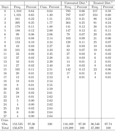
The object of interest is the deaths within the first 28 days after birth. However, since the number of reported deaths are smaller nearer the end of the time period in the treated as well as the untreated districts, we restrict our analysis to modeling the hazard during the first 18 days after birth. Hence, we use 18 days as our censoring point instead of 28 days. The frequency distribution of survival information by treatment status is provided in Table 1: 40,531 babies (24.8%) were born in the districts under treatment. The control group consists of 123,086 babies (75.2%). We also note that (i) the proportion of babies dying in each day is generally lower for babies born in treated districts compared to those born in untreated districts and that (ii) the observed frequencies exhibit heaping at days multiples of 5 in both samples. The model includes various control variables at the parental level as well as the child level. Summary statistics for these variables distinguished by treatment status can be found in Section S5 of the supplementary material.

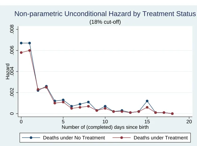
As a preliminary to the estimation of formal models, it is informative to examine the non-parametric estimates of the unconditional discrete hazard function distinguished by the treatment status. These are plotted in Figure 3 and are calculated as the ratio of number of failures during the interval divided by the number of babies alive at the beginning of the interval. All babies born alive and survived the first 18 days are treated as censored observations and are also included in the risk set in the plot. The estimated hazard for those babies born in the treated districts generally lie below the hazard for the control group. Notice however that both the denominator and the numerator suffer from rounding errors and so should be interpreted with care.

Empirical Findings: We estimate the model based on the specification outlined in Section 5. Since heaps in the data appear to be pronounced differently at different days (cf. Table 1), we allow for ‘small’ heaps at days 5 and 10, and for a ‘big’ heap at day 15 in the heaping

20

As the DLHS is representative at the district level, appropriate weights to obtain summary statistics at the district level are provided in the dataset.

21

specification. The former are associated with DH−1 _{={4,9} and D}H+1 _{={6,11} together}

with the probabilities p1 and q1, while the ‘big’ heap is assumed to contain true durations

from {13,14} and {16,17}, respectively. The corresponding probabilities are p1, p2, q1,

and q2, respectively. We setk= 12 relying partially on information from the Program for

Appropriate Technology in Health (PATH) report (2012, p.20) on neonatal mortality in Uttar Pradesh, which suggests that the number of babies dying after 10 days after birth is relatively stable and not subject to large fluctuations.

We start our empirical analysis by testing for the presence of heaping effects (Hπ1_{) via}

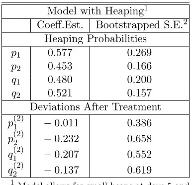
the LR test described in Remark 4.2 of Section 4. The result of this exercise can be found in Table 2, which reports the test statistic as well as the corresponding bootstrapped 95% critical value, and clearly suggests that heaping matters in our model. In fact, examining Table 3, which reports the estimated rounding probabilities together with their deviations for a model that accounts for the introduction of the JSY program, confirms the finding that all heaping parameters are significantly different from zero at conventional levels.

Having established that heaping matters from a statistical point of view, we next turn to the actual analysis of the JSY program: as outlined in Section 5, in a first step we would like to rule out that changes in the reporting behavior (as a result of the policy introduction) confound any observable effect of the program. Therefore, we start by testing Hπ3_{, which under the null postulates that all deviationsp}(2)

1 throughq (2)

2 are jointly equal to

zero. Examining the second row of Table 2, we find that we cannot reject this null on a 5% significance level. This is in line with the standard errors ofp_b(2)₁ ,p_b(2)₂ ,q_b1(2), andq_b(2)₂ in Table 3, which all exceed the size of the actual parameter estimates. Thus, albeit theoretically plausible, our findings do not support the conjecture that mothers who delivered in treated districts reported differently from those in untreated ones (e.g., because births were better recorded).

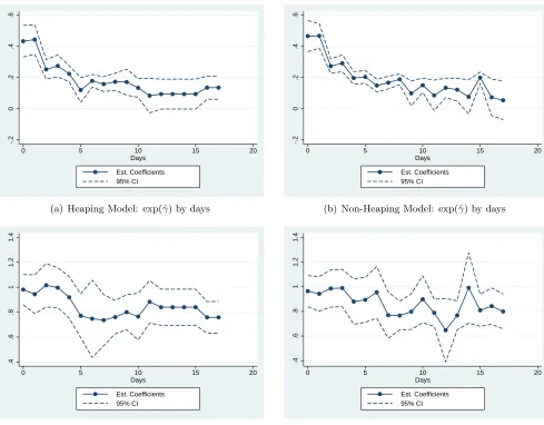
In a second step, we now analyze the effect of the JSY program on the baseline parame-tersγ(0), . . . , γ(17). Figures 4(a) and 4(c) display the estimated coefficients of exp(γ(·)) and exp(γ(2)(·)), respectively, which have been estimated in exponential form. Thus, note that exp(γ(2)(·)) = 1 implies that no change has taken place after the introduction of the policy. Pointwise 95% confidence intervals have been plotted around the coefficient estimates.

While it is straightforward to see from Figure 4(a) that we can reject the null that the (stepwise) integrated baseline hazard is zero for each day except days 11 to 15 at a 5% level (recall thatγ(τ) = lnRτ+1

τ λ0(s)ds), we note that we are only able to reject (again, at a 5% significance level) the null that exp(γ(2)_{(·)) = 1 after day 4.}22 _{However, given that}

the majority of deaths occurs within the first 3 days of birth, this finding can at best be interpreted as weak evidence for a reduction in mortality. In fact, turning back to Table 2, we find that the null ofHγ2_{, which states that at least some of the baseline parameters}

decreased, cannot be rejected at a 5% significance level either.

For comparison reasons, we contrast these results with estimates from a second spec-ification that neglects heaping altogether, see Figures 4(b) and 4(d): while estimates of exp(γ(·)) are generally very similar to the ones displayed in Figure 4(a) (a notable excep-tion are days 10 and 15), we point out that there are some differences in the estimates of

22

Judging by Figure 4(c), it is also clear that the null of the testHγ1_{, which postulates that no uniform}

exp(γ(2)(·)) particularly around days 5 and 10, which indicate a significant reduction in the model that takes account of the heaping, but not in the one that ignores heaping altogether. Summarizing the findings of this section, we note that our estimates and testHπ1 _suggest

clear evidence of heaping in the data. By contrast, our test results do not indicate that the introduction of the JSY program led to a significant reduction in mortality over the first 18 days after birth. That is, while some estimated coefficients of exp(γ(2)(·)) indicated a significant reduction of mortality for days 5, 7 to 10, and 12 onwards, we were not able to confirm this finding through a joint hypothesis test on all coefficients as we cannot reject the null of all parameters jointly equal to zero at a 5% significance level (cf. Hγ2_).

However, we stress that our analysis was conducted using only those babies born in dis-tricts that were eventually treated, and hence captures the “intention to treat” effect rather than the actual effect of mothers receiving treatment. Thus, it remains to be established whether the latter effect exhibits a similar pattern, too.

7

Conclusions

India has one of the largest neonatal mortality rates in the world. To address this, the Indian Government launched a conditional cash-incentive program (JSY) to encourage in-stitutional delivery in 2005. This paper studied the effect of the program on the neonatal mortality rate. Mortality is modeled using survival analysis, paying special attention to the substantial heaping present in the data. The main methodological contribution of the paper is the provision of a set of sufficient conditions for pointwise identification and consistent estimation of the baseline hazard parameters in the joint presence of heaping and unobserved heterogeneity. Our identification strategy requires neither administrative data nor multiple measurements, but the presence of a correctly reported duration and of some flat segment(s) in the baseline hazard, which includes this correctly reported duration point. Information about the correctly reported duration and the flat segment can stem from different sources and does not need to come from a specific data set. The likelihood is constructed down-weighting the contribution of heaped durations and over-weighting the contribution of non heaped durations. This adjustment ensures consistent estimation of both heaping and baseline hazard parameters, and we establish the asymptotic properties of the maximum likelihood estimator. Moreover, the paper provides various specification tests that allow, among other things, (i) to check for the presence of heaping effects (ii) to compare different heaping specifications (iii) to test for shifts in the baseline hazard.

In the supplementary material, we provide an informal discussion of how the idea of our identification strategy can be straightforwardly extended to cover different discrete duration models (e.g., Han and Hausman, 1990; Sueyoshi, 1995) as well as standard ordered choice models. The identification results are therefore not limited to the model used in Section 2, but can also be applied to non-duration data.

Appendix I

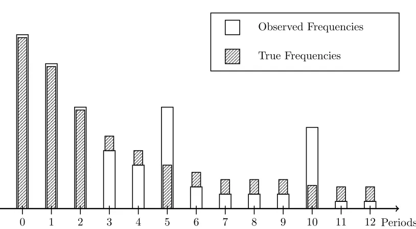
Figure 1: Stylized Failure Frequencies

True Frequencies Observed Frequencies

0 1 2 3 4 5 6 7 8 9 10 11 12 Periods

Note: The figure is a stylized example of a discrete time failure distribution with heaps at time periods 5 and 10. Observed and true frequencies differ from period 3 onwards.

Figure 2: Stylized Heaping Mechanism

7

∈ DH+2

13

∈ DH−2

8

∈ DH−2

9

∈ DH−1

10

∈ DH

11

∈ DH+1

12

∈ DH+2

p2

p1

q2

q1

q2 p2

7

∈ DH+2

8

∈ DH−2

9

∈ DH−1

10

∈ DH

11

∈ DH+1

12

∈ DH+2

13

∈ DH−2

Table 1: Neonatal Mortality− Deaths by Number of Days of Survival

Untreated Dist.1 Treated Dist.1 Days Freq. Percent Cum. Percent Freq. Percent Freq. Percent

0 1,010 0.64 0.64 793 0.66 217 0.58 1 1,021 0.65 1.30 797 0.67 224 0.60

2 341 0.22 1.51 255 0.21 86 0.23

3 395 0.25 1.77 304 0.25 91 0.24

4 179 0.11 1.88 141 0.12 38 0.10

5 188 0.12 2.00 147 0.12 41 0.11

6 99 0.06 2.06 79 0.07 20 0.05

7 124 0.08 2.14 103 0.09 21 0.06

8 153 0.10 2.24 128 0.11 25 0.07

9 43 0.03 2.27 33 0.03 10 0.03

10 101 0.06 2.33 82 0.07 19 0.05

11 33 0.02 2.35 27 0.02 6 0.02

12 37 0.02 2.38 31 0.03 6 0.02

13 16 0.01 2.39 14 0.01 2 0.01

14 27 0.02 2.40 19 0.02 8 0.02

15 165 0.11 2.51 142 0.12 23 0.06

16 20 0.01 2.52 17 0.01 3 0.01

17 12 0.01 2.53 8 0.01 4 0.01

18 18 0.01 2.54

19 8 0.01 2.55

20 65 0.04 2.59

21 28 0.02 2.61

22 18 0.01 2.62

23 5 0.00 2.62

24 4 0.00 2.62

25 24 0.02 2.64

26 6 0.00 2.64

27 4 0.00 2.64

Cens.

Obs. 152.535 97,36 100 116,169 97.38 36,546 97.74

Total 156,679 100 119,289 100 37,390 100

1 _{The treatment status is based on whether at least 18% of the women who gave birth in a}

Figure 3: Unconditional Hazards

0

.002

.004

.006

.008

Hazard

0 5 10 15 20

Number of (completed) days since birth

Deaths under No Treatment Deaths under Treatment

(18% cut-off)

Non-parametric Unconditional Hazard by Treatment Status

Note: The discrete hazard was calculated as the ratio of number of failures during the interval divided by the number of babies alive at the beginning of the interval.

Table 2: Specification Tests1

LR-statistic 95% CV2 Hπ1 298.74 288.29 Hπ3 419.54 619.44 Hγ2 507.83 744.47

1 _{See Sections 4 and 5 for details}

of the hypotheses that are being tested.

2 _{Based on Empirical Bootstrap}

Table 3: Estimated ‘Heaping’ Parame-ters

Model with Heaping1

Coeff.Est. Bootstrapped S.E.2 Heaping Probabilities

p1 0.577 0.269

p2 0.453 0.166

q1 0.480 0.200

q2 0.521 0.157

Deviations After Treatment p(2)₁ −0.011 0.386 p(2)₂ −0.232 0.658 q₁(2) −0.207 0.552 q₂(2) −0.137 0.619

1 _{Model allows for small heaps at days 5 and}

10 with associated probabilitiesp1 and q1,

and a large heap at day 15 with associated probabilitiesp1,p2,q1, andq2.

2

-.2

0

.2

.4

.6

0 5 10 15 20

Days

Est. Coefficients 95% CI

(a) Heaping Model: exp(ˆγ) by days

-.2

0

.2

.4

.6

0 5 10 15 20

Days

Est. Coefficients 95% CI

(b) Non-Heaping Model: exp(ˆγ) by days

.4

.6

.8

1

1.2

1.4

0 5 10 15 20

Days

Est. Coefficients 95% CI

(c) Heaping Model: exp(ˆγ2) by days

.4

.6

.8

1

1.2

1.4

0 5 10 15 20

Days

Est. Coefficients 95% CI

(d) Non-Heaping Model: exp(ˆγ2) by days

Figure 4: Estimated Baseline Hazard and Deviation Coefficients (with pointwise 95% CI)

Appendix II

Proof of Proposition 1: In the following, suppose that the flat segment lies around the last heap j·h∗ and thatk=j·h∗−r−1 andτ =j·h∗+r+ 1. Note that setting the flat region around the last heapj·h∗ comes at no loss of generality since the main steps of the proof remain identical if j < j (see Remark A1 below). We set r = 1, which implies that j·h∗ =k+ 2. The extension to r >1 will be outlined subsequently. Finally, without loss of generality, assume thatzi is a scalar.

Define for any time period τ < τ

H0(τ) =

τ

X

s=0

exp (γ(s))