Anonymous Author 1 Anonymous Author 2 Anonymous Author 3 Unknown Institution 1 Unknown Institution 2 Unknown Institution 3
Abstract
The stochastic knapsack problem is a stochastic resource allocation problem that arises frequently and yet is exceptionally hard to solve. We derive and study an op-timistic planning algorithm specifically de-signed for the stochastic knapsack problem. Unlike other optimistic planning algorithms for MDPs, our algorithm,OpStoK, avoids the use of discounting and is adaptive to the amount of resources available. We achieve this behavior by means of a concentration inequality that simultaneously applies to a capacity and reward estimate. Crucially, we are able to guarantee that the aforementioned confidence regions hold collectively over all time steps by an application of Doob’s in-equality. We demonstrate that the method returns an -optimal solution to the stochas-tic knapsack problem with high probability. To the best of our knowledge, our algorithm is the first which provides such guarantees for the stochastic knapsack problem. Fur-thermore, our algorithm is an anytime algo-rithm and will return a good solution even if stopped prematurely. This is particularly important given the difficulty of the prob-lem. We also provide theoretical conditions to guaranteeOpStoKdoes not expand all poli-cies and demonstrate favorable performance in a simple experimental setting.
1
Introduction
The stochastic knapsack problem (Dantzig, 1957), is a classic resource allocation problem that consists of selecting a subset of items to place into a knapsack of
Preliminary work. Under review by AISTATS 2017. Do not distribute.
a given capacity. Placing each item in the knapsack consumes a random amount of the capacity and pro-vides a stochastic reward. Many real world scheduling, investment, portfolio selection, and planning problems can be formulated as the stochastic knapsack problem. Consider, for instance, a fitness app that suggests a one hour workout to a user. Each exercise (item) will take a random amount of time (size) and burn a random amount of calories (reward). To make optimal use of the available time the app needs to track the progress of the user and adjust accordingly. Once an item is placed in the knapsack, we assume we observe its re-alized size and can use this to make future decisions. This enables us to consider adaptive or closed loop strategies, which will generally perform better (Dean et al., 2008) than open loop strategies in which the schedule is invariant of the remaining budget.
Finding exact solutions to the simpler deterministic knapsack problem, in which item weights and rewards are deterministic, is known to be NP-hard and it has been stated that the stochastic knapsack problem is PSPACE-hard (Dean et al., 2008). Due to the dif-ficulty of the problem, there are currently no algo-rithms that are guaranteed to find satisfactory ap-proximations in acceptable computation time. While ultimately one aims to have algorithms that can ap-proach large scale problems, the current state-of-the-art makes it apparent that the small scale stochas-tic knapsack problem must be tackled first. The em-phasis in this paper is therefore on this small scale stochastic knapsack setting. The current state-of-the-art approaches to the stochastic knapsack problem where the reward and resource consumption distribu-tions are known, were introduced in Dean et al. (2008). Their algorithm groups the available items into small and large items and fills the knapsack exclusively with items of one of the two groups, ignoring potential high reward items in the other group, but still returning a policy that comes within a factor of1/(3+κ)of the
de-cision tree is built to some predefined depth d and an exhaustive search for the best policy in that deci-sion tree is performed. For most non-trivial problems, this tree can be exceptionally large. The notion of small items is also underlying recent work in machine learning where the reward and consumption distribu-tions are assumed to be unknown (Badanidiyuru et al., 2015). The approach in Badanidiyuru et al. (2015) works with a knapsack size that converges (in a suit-able way) to infinity, rendering all items small. The stochastic knapsack problem is also a generalization of the the pure exploration combinatorial bandit prob-lem, eg Chen et al. (2014); Gabillon et al. (2016) It is desirable to have methods for the stochastic knap-sack problem that can make use of all available re-sources and adapt with the remaining capacity. For this, the tree structure from Dean et al. (2008) can be useful. We propose using ideas from optimistic plan-ning (Busoniu and Munos, 2012; Sz¨or´enyi et al., 2014) to significantly accelerate the tree search approach and find adaptive strategies. Most optimistic planning al-gorithms were developed for discounted MDPs and as such rely on discount factors to limit future reward, ef-fectively reducing the search tree to a tree with small depth. However, these discount factors are not present in the stochastic knapsack problem. Furthermore, in our problem, the random variable representing state transitions also provides us with information on the future rewards. To avoid the use of discount factors and use the transition information, we work with con-fidence bounds that incorporate estimates of the re-maining capacity and use these estimates to determine how many samples we need. For this, we need tech-niques that can deal with weak dependencies and that give us confidence regions that hold simultaneously for multiple sample sizes. We therefore combine Doob’s martingale inequality with Azuma-Hoeffding bounds to create our high probability bounds. Following the optimistic planning approach, we use these bounds to develop an algorithm that adapts to the complexity of the problem instance: in contrast to the current state-of-the-art, it is guaranteed to find an-good ap-proximation independent of how difficult the problem is and, if the problem instance is easy to solve, it ex-pands only a moderate sized tree. Our algorithm is also an ‘anytime’ algorithm in the sense that, it im-proves rapidly to begin with and if stopped prema-turely, it will still return a good solution. For our al-gorithm, we only require access to a generative model of item sizes and rewards, and no further knowledge of the distributions.
We measure the performance of our algorithm in terms of the number of policies it expands. In a theoretical manner we define the set of-critical policies to be the
set of policies an algorithm may expand to obtain a solution within of the optimal. We also show that, in practice, the number of policies explored by our algorithm OpStoK is small and compares favorably to that of the algorithm from Dean et al. (2008).
1.1 Related work
Due to the difficulty of the stochastic knapsack prob-lem, the main approximation algorithms focus on the variant of the problem with deterministic sizes and stochastic rewards (eg. Steinberg and Parks (1979) and Morton and Wood (1998)), or stochastic sizes and deterministic rewards (eg. Dean et al. (2008) and Bhalgat et al. (2011)). Of these, the most relevant to us are Dean et al. (2008) and Bhalgat et al. (2011) where decision trees are used to obtain approximate adaptive solutions to the problem. To limit the size of the decision tree Dean et al. (2008) use a greedy strategy for ‘small’ items while Bhalgat et al. (2011) group items together in blocks. Morton and Wood (1998) use a Monte-Carlo sampling strategy to gen-erate a non-adaptive (open loop) solution in the case with stochastic rewards and deterministic sizes. The bandits with knapsacks problem of Badanidiyuru et al. (2015) is different to ours since it does not re-quire access to a generative model of item sizes and rewards but learns the distributions by playing items multiple times. This requires a large budget and the resulting strategies are not adaptive. In Burnetas et al. (2015) adaptive strategies are considered for determin-istic item sizes and renewable budgets.
algo-rithm of Gabillon et al. (2012).
There are several key differences between our problem and the MDPs optimistic planning algorithms are typ-ically designed for. Generally, in optimistic planning it is assumed that the state transitions do not pro-vide any information about future reward. However, in our problem this information is relevant and should be considered when defining the high confidence bounds. Furthermore, optimistic planning algorithms are used to approximate complex systems at just one point and return a near optimal first action. In our case, the deci-sion tree is a good approximation to the entire problem so we can output a near-optimal policy. Furthermore, to the best of our knowledge, our algorithm is the first optimistic planning algorithm to iteratively build con-fidence bounds which are used to determine whether it is necessary to sample more. One would imagine that the StOP algorithm from Sz¨or´enyi et al. (2014) could be easily adapted to the stochastic knapsack problem. However, as discussed in Section 4.1, the assumptions required for this algorithm to terminate are too strong for it to be considered feasible for this problem.
1.2 Our contribution
Our main contributions are the anytime algo-rithm OpStoK (Algorithm 1)) and subroutine
BoundValueShare (Algorithm 2). These are sup-ported by the confidence bounds in Lemma 1 and Proposition 2 that allow us to simultaneously esti-mate remaining capacity and reward with guarantees that hold uniformly over multiple sample sizes, and Proposition 3, which shows that we can avoid discount based arguments and still return an adaptive policy with value within of the optimal policy, with high probability and while using adaptive capacity estimates. This makes OpStoK the first algorithm to provably return an-optimal solution. Theorem 5 and Corollary 6 provide bounds on the number of samples our algorithm uses in terms of how many policies are -close to the best policy. The empirical performance of OpStoKis then discussed in Section 7.
2
Problem formulation
We consider the problem of selecting a subset of items from a set of K items, I, to place into a knapsack of capacity B where each item can be played at most once. For each item i∈I, let Ci and Ri be bounded random variables defined on a joint probability space (Ω,A, P) which represent the size and reward of item i. It is assumed that we can simulate from the gen-erative model of (Ri, Ci) for alli∈I and we will use lower caseci andri, to denote realizations of the ran-dom variables. We assume that the ranran-dom variables
(Ri, Ci) are independent of (Rj, Cj) for all i, j ∈ I, i 6= j. Further, it is believed that item sizes and re-wards do not change dependent on the other items in the knapsack. We assume the problem is non-trivial, in the sense that it is not possible to fit all items in the knapsack at once. If we place an item i in the knapsack and the consumption Ci is strictly greater than the remaining capacity then we gain no reward for that item. Our final important assumption is that there exists some non-decreasing function Ψ(·), satis-fying limb→0Ψ(b) = 0 and Ψ(B)<∞, such that the
reward that can be achieved with budget b is upper bounded by Ψ(b).
Representing the stochastic knapsack problem as a tree requires that all item sizes take discrete values. While in this work, it will generally be assumed that this is the case, in some problem instances, continu-ous item sizes need to be discretized. In this case, let ξ∗ be the discretization error of the optimal policy. Then Ψ(ξ∗) is an upper bound on the extra reward that could be gained from the space lost due to dis-cretization. For discrete sizes, we assume there are s possible values the random variable can take and that there existsθ >0 such thatCi ≥θ for alli∈I. 2.1 Planning trees and policies
The stochastic knapsack problem can be thought of as a planning tree with the initial empty state as the root at level 0. Each node on an even level is an ac-tionnode and its children represent placing an item in the knapsack. The nodes on odd levels are transition nodes with children representing item sizes. We define a policy Π as a finite subtree where each action node has at most one child and each transition node has s children. The depth of a policy Π,d(Π), is defined as the number of transition nodes in any realization of the policy (where each transition node has one child), or equivalently, the number of items. Let d∗ =bB/θcbe the maximal depth of any policy. For any 1≤d≤d∗, the number of policies of depth dis,
Nd= d−1
Y
i=0
(K−i)si (1)
whereK=|I|is the number of items, andsthe num-ber of discrete sizes.
for another item to be inserted into the knapsack (see Section 4.2 for a formal definition).
The value of a policy Π can be defined as the cumu-lative expected reward obtained by playing items ac-cording to Π, VΠ =P
T
t=1E[Rit] where it is the t-th item chosen by Π. LetP be the set of all policies, then define theoptimal policy as Π∗= arg maxΠ∈PVΠ, and
correspondingoptimal valueasv∗= maxΠ∈PVΠ. Our
algorithm returns an-optimalpolicy with valuev∗−. For any policy Π, we define a sample of Π as follows. The first item of any policy is fixed so we take a sam-ple of the reward and size from the generative model of that item. We then use Π to tell us which item to sample next (based on the size of the previous item) and sample the reward and size of that item. This continues until the policy finishes or the cumulative sampled sizes of the selected items exceeds B.
3
High confidence bounds
In this section, we develop confidence bounds for the value of a policy. Observe that a policy Π need not consume all available budget, in fact our algorithm will construct iteratively longer policies starting from the shortest policies of playing a single item. Con-sequently, we are also interested in R+Π, the expected maximal reward that can be obtained after playing ac-cording to policy Π until all budget is consumed. Let BΠ be a random variable representing the remaining
budget after playing according to a policy Π. Our assumptions guarantee that there exists a function Ψ such that R+Π ≤ EΨ(BΠ). We define VΠ+ to be the
maximal expected value of any continuation of policy Π soVΠ+=VΠ+R+Π≤VΠ+EΨ(BΠ).
From m samples of the reward of policy Π, we esti-mate the value of Π as VΠm = m1
Pm
j=1
Pd(Π)
d=1 r (j)
i(d),
where ri((jd))is the reward of itemi(d) chosen at depth d of sample j. However, our real interest is in the value of VΠ+ since we wish to identify the pol-icy with greatest reward when continued until the budget is exhausted. From Hoeffding’s inequality, P
|VΠm1−V
+
Π|> EΨ(BΠ) +
q
Ψ(B)2log(2/δ)
2m
≤ δ.
This bound depends on the quantityEΨ(BΠ) which is
typically not known. The following lemma shows how our bound can be improved by independently sam-pling Ψ(BΠ) m times to get samples ψ1, . . . , ψm and
estimating Ψ(BΠ)m= m1 Pmj=1ψj.
Lemma 1 Let (Ω,A, P)be the probability space from Section 2, then for m1+m2 independent samples of
policy Π, andδ1, δ2>0, with probability1−δ1−δ2,
VΠm1−k1≤V
+
Π ≤VΠm1+ Ψ(BΠ)m2+k1+k2.
Where, k1:=
qΨ(B)2log(2/δ
1)
2m1 ,k2:=
qΨ(B)2log(1/δ
2)
2m2 .
We will not use the bound in this form since our al-gorithm will work by sampling Ψ(BΠ) until we are
confident enough that it is small or large. This in-troduces weak dependencies into the sampling pro-cess so we need guarantees to hold simultaneously for multiple sample sizes, m2. For this, we work with
martingale techniques and use Azuma-Hoeffding like bounds (Azuma, 1967), similar to the technique used in Perchet et al. (2016). Specifically, in Lemma 8 (sup-plementary material), we use Doob’s maximal inequal-ity and a peeling argument to get Azuma like bounds for the maximal deviation of the sample mean from the expectation under boundedness. Assuming we sample the reward of a policy m1 times and the remaining
capacitym2 times, the following key result holds.
Proposition 2 The Algorithm BoundValueShare (Algorithm 2) returns confidence bounds,
L(VΠ+) =VΠm1−c1
U(VΠ+) =VΠm1+ Ψ(BΠ)m2+c1+c2
which hold with probability 1−δ1−δ2, where
c1=
q
Ψ(B)2log(2/δ1)
2m1 , c2= 2Ψ(B)
r
1
m2log
8n δ2m2
.
This upper bound depends onn, the maximum num-ber of samples of Ψ(BΠ). For any policy Π, the
mini-mum width a confidence interval of Ψ(BΠ) created by BoundValueSharewill ever need to be is/4. Taking,
n=
162Ψ(B)2log(8/δ)
2
, (2)
ensures that for all policies, 2c2 ≤/4 when m2 =n.
This is a necessary condition for the termination of our algorithm, OpStoK, as will be discussed in Section 4.2
4
Algorithms
Before presenting our algorithm for optimistic plan-ning of the stochastic knapsack problem, we first dis-cuss a simple adaptation of the algorithm StOP from Sz¨or´enyi et al. (2014).
4.1 Stochastic optimistic planning for knapsacks
One naive approach to optimistic planning in the stochastic knapsack problem is to adapt the algorithm
be achieved without using sample of item sizes. The upper bound on VΠ+is thenVΠm+ Ψ(B−dθ) +c, for m samples and confidence bound c. With this, most of the results from Sz¨or´enyi et al. (2014) follow fairly naturally. AlthoughStOP-Kappears to be an intuitive extension of StOP to the stochastic knapsack setting, it can be shown that for a finite number of samples, unless Ψ(B −θd∗) ≤
2, the algorithm will not
ter-minate. As such, unless this restrictive assumption is satisfied StOP-Kwill not converge.
4.2 Optimistic stochastic knapsacks
In the stochastic knapsack problem, the process of sampling the reward of a policy involves sampling item sizes to decide which item to play next. We propose to make better use of this data by using the samples of item sizes to calculateU(Ψ(BΠ)) which is then
incor-porated intoU(VΠ+). Instead of the worst case bound Ψ(B −dθ), our algorithm, OpStoK, uses the tighter upper bound U(Ψ(BΠ)). We also pool samples of the
reward and size of items across policies, thus reducing the number of calls to the generative model. OpStoK
benefits from an adaptive sampling scheme that re-duces sample complexity and ensures that an entire -optimal policy is returned when the algorithm stops (line 5, Algorithm 1). This is achieved by using the bound in Proposition 2 and nas defined in (2). In the main algorithm, OpStoK(Algorithm 1) is very similar to StOP-K Sz¨or´enyi et al. (2014) with the key differences appearing in the sampling and con-struction of confidence bounds which are defined in
BoundValueShare. OpStoK proceeds by maintaining a set of ‘active’ policies. As in Sz¨or´enyi et al. (2014) and Gabillon et al. (2012), at each time step t, a pol-icy, Πt to expand is chosen by comparing the upper confidence bounds of the two best active policies. We select the policy with most uncertainty in the bounds since we want to be confident enough in our estimates of the near-optimal policies to say that the policy we ultimately select is better (see Figure 4, supplemen-tary material). Once we have selected a policy, Πt, if the stopping criteria is not met, we replace Πt in the set of active policies with all its children. For each child policy, we use BoundValueShare to bound its reward. In order for all our bounds to hold simulta-neously with probability greater than 1−δ0,1−δ0,2
(as shown in Lemma 12, supplementary material),
BoundValueSharemust be called with parameters
δd,1=
δ0,1
d∗ N −1
d(Π) and δd,2=
δ0,2
d∗ N −1
d(Π) (3)
where Nd is the number of policies of depth d as given in (1). Our algorithm, OpStoK is given in Al-gorithm 1. The alAl-gorithm relies on BoundValueShare
(Algorithm 2) and subroutines,EstimateValue (Algo-rithm 3, supplementary material) and SampleBudget
(Algorithms 4, supplementary material), which sample the reward and budget of policies.
InBoundValueShare, we use samples of both item size and reward to bound the value of a policy. We define upper and lower bounds on the value of any extension of a policy Π as,
U(VΠ+) =VΠm1+ Ψ(BΠ)m2+c1+c2,
L(VΠ+) =VΠm1−c1,
with c1 and c2 as in Proposition 2. It is also
possi-ble to define upper and lower bounds on Ψ(BΠ) with
m2 samples and confidence δ2. From this, we can
formally define a complete policy as a policy Π with U(BΠ) = Ψ(BΠ)m2 +c2 ≤ 2. For complete policies,
since there is very little capacity left, it is more im-portant to get tight confidence bounds on the value of the policy. Hence, in BoundValueShare, we sample the remaining budget of a policy as much as is nec-essary to conclude whether the policy is complete or not. As soon as we realize we have a complete pol-icy (U(BΠ)≤/2), we sample the value of that policy
sufficiently to get a confidence interval of width less than . Then, when it comes to choosing an optimal policy to return, the confidence intervals of all com-plete policies will be narrow enough for this to happen. This is appropriate since, pre-specifying the number of samples may not lead to confidence bounds tight enough to select an-optimal policy. Furthermore, this method will focus sampling efforts only on promising policies that are near completion. If a complete policy is chosen as Π(1)t inOpStoK, for somet, the algorithm will stop and this policy will be returned. For this to happen, we also need the stopping criterion to be checked before selecting a policy to expand. Note that in BoundValueShare, the reward and remaining bud-get must be sampled separately as we are considering closed-loop planning so the item chosen may depend on the size of the previous item, and hence the re-ward will depend on the instantiated item sizes. In line 6 of BoundValueShare, for an incomplete policy, the number of samples of the reward, m1, is defined
to ensure that the uncertainty in the estimate of VΠ
is less than u(Ψ(B)) = min{U(Ψ(BΠ)),Ψ(B)}, since
Algorithm 1: OpStoK(I, δ0,1, δ0,2, )
Initialization:Active=∅
1 forall thei∈I do
2 Πi= policy consisting of just playing itemi.
3 d(Πi) = 1
4 δ1,1=
δ0,1
d∗ N −1
1 δ1,2=
δ0,2
d∗N −1 1
5 (L(VΠ+ i), U(V
+
Πi)) = BoundValueShare (Πi, δ0,1, δ0,2,S∗, )
6 Active=Active∪ {Πi}.
7 end
8 fort= 1,2, . . . do
9 Π(1)t = arg maxΠ∈ActiveU(V + Π)
10 Π(2)t = arg max
Π∈Active\{Π(1)t } U(VΠ+)
11 if L(V+
Π(1)t ) +≥maxΠ∈ActiveU(V + Π)then
12 Stop: Π∗= Π(1)t ;
13 Πt= Π(a
∗)
t , where a∗= arg max
a∈{1,2}U(Ψ(BΠ(ta)))
14 Active=Active\ {Πt}
15 forall thechildren Π0 ofΠt do
16 d(Π0) =d(Πt) + 1
17 δ1=δd0∗,1N −1
d(Π0)andδ2=δd0∗,2N −1
d(Π0)
18 (L(VΠ+0), U(VΠ+0)) =BoundValueShare
(Π0, δ1, δ2,S∗, )
19 Active=Active∪ {Π0}
20 end
21 end
and so will be a good policy (or beginning of policy).
OpStoK, also considerably reduces the number of calls to the generative model by creating setsSi∗of samples of the reward and size of each item i∈I. When it is necessary to sample the reward and size of an item for the evaluation of a policy, we sample without replace-ment fromS∗
i, until|Si∗|samples have been taken. At this point new calls to the generative model are made and the new samples added to the sets for use by future policies. This is illustrated in EstimateValue (Algo-rithm 3, supplementary material) and SampleBudget
(Algorithm 4, supplementary material). We denote by
S∗the collection of all sets S∗
i.
5
-critical policies
The set of-critical policies is the set of all policies an algorithm may potentially expand in order to obtain an-optimal solution. The number of-critical policies in this set represents a bound on the number of policies an algorithm may explore in order to obtain this -optimal solution.
To define the set of -critical policies associated with
Algorithm 2: BoundValueShare(Π, δ1, δ2, S∗, )
Input: Π: policy; δ1: probability capacity confidence
bound fails; δ2: probability reward confidence
bound fails; S∗: observed samples for all items;: tolerated approximation error. Initialization: For alli∈I, letSi=Si∗
1 Setm2= 1 and (ψ1,S) =SampleBudget(Π,S) /* draw a sample of the remaining budget */
2 Ψ(BΠ)m2 =
1
m2
Pm2
j=1ψj
3 U(Ψ(BΠ)) = Ψ(BΠ)m2+ 2Ψ(B)
r
1
m2log
8n δm2
,
L(Ψ(BΠ)) = Ψ(BΠ)m2−2Ψ(B)
r
1
m2log
8n δm2
/* calculate upper and lower bounds on the
remaining budget */
4 if U(Ψ(BΠ))≤2 then m1=
l8Ψ(B)2log(2/δ 1)
2
m
;
5 else if L(Ψ(BΠ))≥4 then
6 m1=
l
1 2
Ψ(B)2log(2/δ 1)
u(Ψ(B))2
m
7 else
8 Setm2=m2+ 1,
(ψm2,S) =SampleBudget(Π,S) and go back to 2
9 VΠm1 =EstimateValue(Π, m1)
10 L(VΠ+) =VΠm1−
q
Ψ(B)2log(2/δ 1)
2m1
11 U(VΠ+) =VΠm1+ Ψ(BΠ)m2+
q
Ψ(B)2log(2/δ 1)
2m1 +
2Ψ(B)
r
1
m2log
8n δm2
12 return (L(VΠ+), U(VΠ+))
OpStoK, let
Q
IC={Π;VΠ+ 6EΨ(BΠ)−3/4≥v∗
−6EΨ(BΠ) +3/4+}
and Q
C={Π;VΠ+≥v∗},
represent the set of potentially optimal incomplete and complete policies. The set of all -critical policies is then Q = Q
IC
S
Q
C. The following lemma then shows that all policies expanded by OpStoKare inQ. Lemma 3 For any policy Π ∈ Active assume that L(VΠ+) ≤ VΠ ≤ U(VΠ+) holds simultaneously for all
policies in the active set with U(VΠ+) and L(VΠ+) as defined in Proposition 2. Then,Πt∈ Qat every time point t considered by the algorithmOpStoK, except for possibly the last one.
con-ditions, OpStoKwill not expand all policies (although in practice this claim should hold even when some of the assumptions are violated). From considering the definition ofQ
IC from Section 6, it can be shown that if there exists a subsetI0 of items andλ >0 satisfying,
X
i∈I0
E[Ri]< v∗−, and,
E
"
Ψ B−X
i∈I0
Ci
!#
< 5 24 +
λ 12
(4)
then Q
IC is a proper subset of all incomplete policies and as such, not all incomplete policies will need to be evaluated byOpStoK. Furthermore, since any policy of depth d >1 will only be evaluated byOpStoKif a de-scendant of it has previously been evaluated, it follows that a complete policy inQ
Cmust have an incomplete descendant in Q
IC. Therefore, sinceQIC is not equal to the set of all incomplete policies,Q
C will also be a proper subset of all complete policies and so Q
(P.
Note that the bounds used to obtain these conditions are worst case as they involve assuming the true value of Ψ(Bπ) lies at one extreme of the confidence interval. Hence, even if the conditions in (4) are not satisfied, it is unlikely that OpStoKwill evaluate all policies. The conditions in (4) are easily satisfied. Consider, for example, the problem instance where= 0.05,Ψ(b) = b ∀0≤b≤B, v∗= 1 andB = 1. Assume there are 3
items i1, i2, i3 ∈I withE[Ri]<1/8 andE[Ci] =8/25.
Then if I0 = {i1, i2, i3} and λ = 5/8, the conditions
of (4) are satisfied and OpStoK will not evaluate all policies.
6
Analysis
In this section we state some theoretical guarantees on the performance of OpStoK with the proofs of all results given in Appendix C.2. We begin with the consistency result:
Proposition 4 With probability at least (1−δ0,1 −
δ0,2), the algorithm OpStoK returns an action with
value at least v∗−for >0.
To obtain a bound on the sample complexity of
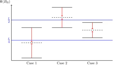
OpStoK, we return to the definition of-critical policies from Section 5. The set of -critical policies, Q, can be represented as the union of three disjoint sets,Q=
A∪B∪C, as illustrated in Figure 1 whereA={Π∈
Q|EΨ(B
Π)≤/4},B={Π∈ Q|EΨ(BΠ)≥/2}and
C = {Π ∈ Q|/
4 < EΨ(BΠ) < /2}. Using this, in
Theorem 5 the total number of samples of item size or reward required byOpStoKcan be bounded as follows. Theorem 5 With probability greater than1−δ0,2, the
total number of samples required byOpStoKis bounded
2
4
Case 1 Case 2 Case 3
[image:7.612.350.544.74.188.2]Ψ(BΠ)
Figure 1: The three possible cases of EΨ(BΠ). In
the first case, EΨ(BΠ)≤ 4 so Π∈ A, in the second
case EΨ(BΠ) ≥ 2 so Π ∈ B
, and in the final case
4 < EΨ(BΠ)< 2 so Π∈ C
.
from above by,
X
Π∈Q
(m1(Π) +m2(Π))d(Π).
Where, for Π∈ A, m
1(Π) =8Ψ(B)2log(δd(Π)2 ,1)/ 2,
forΠ∈ B, m
1(Π)≤Ψ(B)2log(δd(Π)2 ,1)/2EΨ(BΠ)2
,
and forΠ∈ C, m
1(Π)≤max
8Ψ(B)2log( 2
δd(Π),1)/ 2,
2Ψ(B)2log( 2
δd,1)/EΨ(BΠ)2 .
And m2(Π) = m∗, where m∗ is the smallest integer
satisfying,
32Ψ(B)2/(EΨ(BΠ)−/2)2≤m/log(4n/mδ2)forΠ∈ A
,
32Ψ(B)2
/(EΨ(BΠ)−/4)2≤m/log(4n/mδ2)forΠ∈ B, 32Ψ(B)2/(/4)2≤m/log(4n/mδ2)forΠ∈ C
.
In order to bound the number of calls to the generative model, we consider the expected number of times item i needs to be sampled by a policy Π. Let i1, . . . , iq
denote theqnodes in policy Π where itemiis played. Then for each node ik(1 ≤ k ≤ q), denote by ζik the unique route to node ik. Define d(ζik) to be the depth of nodeik, or the number of items played along routeζik. Then the probability of reaching nodeik(or taking route ζik) is P(ζik) =Q
d(ζik)
`=1 p`,Π(ik,`), where ik,` denotes the`th item on the route to itemik and, pl,Π(ij) is the probability of choosing itemij at depth
l of policy Π. Denote the probability of playing itemi in policy Π byPΠ(i), then,PΠ(i) =Pqk=1P(ζik). Us-ing this, the expected number of samples of the reward and size of item i required by policy Π are less than m1(Π)PΠ(i), andm2(Π)PΠ(i) respectively. Since
sam-ples are shared between policies, the expected number of calls to the generative model of item i is as given below and used in Corollary 6,
M(i)≤ max
Π∈Q
max{m1(Π)PΠ(i), m2(Π)PΠ(i)}
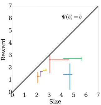
Figure 2: Item sizes and rewards. Each color repre-sents an item with horizontal lines between the two possible sizes and vertical lines between minimum and maximum reward. The lines cross at the point (mean size, mean reward).
Corollary 6 The expected total number of calls to the generative model byOpStoK for a stochastic knap-sack problem of K items is bounded from above by
PK
i=1M(i).
7
Experimental results
We demonstrate the performance of OpStoKon a sim-ple experimental setup with 6 items. Each item ican take two sizes with probability xi, and the rewards come from scaled and shifted Beta distributions. The budget is 7 meaning that a maximum of 3 items can be placed in the knapsack. We take Ψ(b) =b and set the parameters of the algorithm to δ0,1 = δ0,2 = 0.1
and= 0.5. Figure 2 illustrates the problem.
We compare the performance ofOpStoKin this setting to the algorithm in Dean et al. (2008) with various val-ues ofκ, the parameter used to define the small items limit. We choseκto ensure that we consider all cases from 0 small items to 6 small items. Note that the algorithm in Dean et al. (2008) is designed for deter-ministic rewards so in order to apply it to our problem, we sampled the rewards for each item at the start and then used the estimates as true rewards. When it came to evaluating the value of a policy, we re-sampled the final policies as discussed in Section 2.1. The results of this experiment are shown in Figure 3. From this, the anytime property of our algorithm can be seen; it is able to find a good policy early on (after less than 100 policies) so if it was stopped early, it would still return a policy with a high expected reward. Furthermore, at termination, the algorithm is very close to the best solution from Dean et al. (2008) which required more
Figure 3: Num policies vs reward. The blue line is the best reward of the best policy so far found by
OpStoK with a square where it terminates. The green diamonds are the best reward for the algorithm from Dean et al. (2008) when small items are chosen, and red circles when it chooses large items. The mean re-ward of the best solution from Dean et al. (2008) is given by the red dashed line.
than twice as many policies to be evaluated. Thus this experiment has shown that our algorithm not only re-turns a policy with near optimal value, it does this af-ter evaluating significantly fewer policies and can even be stopped prematurely to return a good policy. These experimental results were obtained using the
OpStoK algorithm as stated in Algorithm 1. This al-gorithm incorporates the sharing of samples between policies and preferential sampling of complete policies to improve performance. For large problems, the com-putational performance of OpStoKcan be further im-proved by parallelization. In particular, the expansion of a policy can be done in parallel with each leaf of the policy being expanded on a different core and then re-combined. It is also possible to sample the reward and remaining budget of a policy in parallel.
8
Conclusion
In this paper we have presented a new algorithm
OpStoK, an anytime optimistic planning algorithm specifically tailored to the stochastic knapsack prob-lem. For this algorithm, we provide confidence inter-vals, consistency results, bounds on the sample size and show that it needn’t evaluate all policies to find an -optimal solution; making it the first such algo-rithm for the stochastic knapsack problem. By using estimates of the remaining budget and reward,OpStok
[image:8.612.112.274.67.235.2]References
P. Auer, N. Cesa-Bianchi, and P. Fischer. Finite-time analysis of the multiarmed bandit problem.Machine Learning, 47(2-3):235–256, 2002.
K. Azuma. Weighted sums of certain dependent ran-dom variables. Tohoku Math. J. (2), 1967.
A. Badanidiyuru, R. Kleinberg, and A. Slivkins. Bandits with knapsacks. In arXiv preprint arXiv:1305.2545, 2015.
A. Bhalgat, A. Goel, and S. Khanna. Improved ap-proximation results for stochastic knapsack prob-lems. In Proceedings of the twenty-second annual ACM-SIAM symposium on Discrete Algorithms, pages 1647–1665. SIAM, 2011.
S. Bubeck and R. Munos. Open loop optimistic plan-ning. InConference on Learning Theory, pages 477– 489, 2010.
A. N. Burnetas, O. Kanavetas, and M. N. Kate-hakis. Asymptotically optimal multi-armed ban-dit policies under a cost constraint. arXiv preprint arXiv:1509.02857, 2015.
L. Busoniu and R. Munos. Optimistic planning for markov decision processes. In 15th International Conference on Artificial Intelligence and Statistics, volume 22, pages 182–189, 2012.
S. Chen, T. Lin, I. King, M. R. Lyu, and W. Chen. Combinatorial pure exploration of multi-armed ban-dits. In Advances in Neural Information Processing Systems, pages 379–387, 2014.
P.-A. Coquelin and R. Munos. Bandit algorithms for tree search. arXiv preprint arXiv:cs/0703062, 2007. G. B. Dantzig. Discrete-variable extremum problems.
Operations Research, 5(2):266–288, 1957.
B. C. Dean, M. X. Goemans, and J. Vondr´ak. Ap-proximating the stochastic knapsack problem: The benefit of adaptivity.Mathematics of Operations Re-search, 33(4):945–964, 2008.
E. Even-Dar, S. Mannor, and Y. Mansour. Action elimination and stopping conditions for the multi-armed bandit and reinforcement learning problems. The Journal of Machine Learning Research, 7:1079– 1105, 2006.
V. Gabillon, M. Ghavamzadeh, and A. Lazaric. Best arm identification: A unified approach to fixed bud-get and fixed confidence. In Advances in Neural Information Processing Systems, pages 3212–3220, 2012.
V. Gabillon, A. Lazaric, M. Ghavamzadeh, R. Ortner, and P. Barlett. Improved learning complexity in combinatorial pure exploration bandits. In19th In-ternational Conference on Artificial Intelligence and Statistics, pages 1004–1012, 2016.
A. Garivier and E. Kaufmann. Optimal best arm identification with fixed confidence. arXiv preprint arXiv:1602.04589, 2016.
J.-F. Hren and R. Munos. Optimistic planning of de-terministic systems. In Recent Advances in Rein-forcement Learning, pages 151–164. Springer, 2008. L. Kocsis and C. Szepesv´ari. Bandit based monte-carlo planning. InEuropean Conference on Machine Learning, pages 282–293. 2006.
D. P. Morton and R. K. Wood. On a stochastic knap-sack problem and generalizations. Springer, 1998. V. Perchet, P. Rigollet, S. Chassang, and E. Snowberg.
Batched bandit problems. The Annals of Statistics, 44(2):660–681, 2016.
A. Sabharwal, H. Samulowitz, and C. Reddy. Guid-ing combinatorial optimization with uct. In Inte-gration of AI and OR Techniques in Contraint Pro-gramming for Combinatorial Optimzation Problems, pages 356–361. Springer, 2012.
E. Steinberg and M. Parks. A preference order dynamic program for a knapsack problem with stochastic rewards. Journal of the Operational Re-search Society, pages 141–147, 1979.
B. Sz¨or´enyi, G. Kedenburg, and R. Munos. Optimistic planning in markov decision processes using a gen-erative model. In Advances in Neural Information Processing Systems, pages 1035–1043, 2014.