Aggregation of Markov flows I : theory

warwick.ac.uk/lib-publications

Original citation:

MacKay, Robert S. and Robinson, J. D. (2018) Aggregation of Markov flows I :

theory. Philosophical Transactions A: Mathematical, Physical and Engineering Sciences, 376

(2118). doi:10.1098/rsta.2017.0232

Permanent WRAP URL:

http://wrap.warwick.ac.uk/97255

Copyright and reuse:

The Warwick Research Archive Portal (WRAP) makes this work of researchers of the University of Warwick available open access under the following conditions. Copyright © and all moral rights to the version of the paper presented here belong to the individual author(s) and/or other copyright owners. To the extent reasonable and practicable the material made available in WRAP has been checked for eligibility before being made available.

Copies of full items can be used for personal research or study, educational, or not-for-profit purposes without prior permission or charge. Provided that the authors, title and full bibliographic details are credited, a hyperlink and/or URL is given for the original metadata page and the content is not changed in any way.

Publisher statement:

First published by Royal Society of Chemistry 2018 http://dx.doi.org/10.1098/rsta.2017.0232

A note on versions:

The version presented here may differ from the published version or, version of record, if you wish to cite this item you are advised to consult the publisher’s version. Please see the ‘permanent WRAP URL’ above for details on accessing the published version and note that access may require a subscription.

R.S.MACKAY AND J.D.ROBINSON

Abstract. A Markov flow is a stationary measure, with the associated flows and mean first passage times, for a continuous-time regular jump homogeneous semi-Markov pro-cess on a discrete state-space. Nodes in the state-space can be eliminated to produce a smaller Markov flow which is a factor of the original one. Some improvements to elim-ination methods of Wales are given. The main contribution of the paper is to present an alternative, namely a method to aggregate groups of nodes to produce a factor. The method can be iterated to make hierarchical aggregation schemes. The potential benefits are efficient computation, including recomputation to take into account local changes, and insights into the macroscopic behaviour.

Keywords: Markov flow, aggregation methods, clustering, model reduction

1. Introduction

Aggregation of Markov processes is an old theme, e.g. [AS], and so is the philosophy of hierarchical aggregation [Si]. Yet, many of the schemes of which we are aware (e.g. [St]) do not look as efficient or accurate as they could be.

The idea of aggregation of a Markov process is to cluster selected nodes into groups and devise an effective Markov process between the groups, that preserves aspects of the group-scale dynamics (also known as “lumping” [KS]). Hierarchical aggregation iterates this procedure to make a hierarchy of descriptions of the same system at successively coarser levels.

Potential outcomes are insight into the macroscopic behaviour, and efficient ways to compute quantities for the system, including efficient re-computation if parts of the system are changed.

There is much active research on aggregation methods more broadly (e.g. see [M]), under names like algebraic multigrid [Wa], coarse-graining [Sh], multilevel or multi-scale analysis [EELRV], lumpability or lumping (e.g. in chemical kinetics [LLJ]), modular decomposition [Il], agglomerative clustering [FVH], homogenisation theory [Al], model reduction (as this special issue), dimension reduction [Cu], highway hierarchies [SS], re-cursive block LU decomposition [DHS, GW], hierarchical incomplete LU decomposition [Saad], scaling laws and renormalisation (e.g. the series [M91, M95, CM] on Frenkel-Kontorova models), and upscaling [OZ]. Many of the methods introduce approxima-tions. Nevertheless, highway hierarchies and the well established Kron reduction [DB] for steady AC power flows (also known as Gauss-Rutishauser elimination or Ward equiv-alent [MBB]) are exact, as are the above cited methods for Frenkel-Kontorova chains, and so is recursive block LU decomposition.

Date: January 6, 2018.

We say an aggregation method is exact if it produces a factor of the original system. A factor of a system A is a system B with a map h from A onto B such that the image under h of a solution for A is a solution for B. In dynamical systems theory, such a map h is called a semi-conjugacy. The application of h to a solution in other contexts requires interpretation. For example, for Markov flows to be addressed here, the stationary measure at a node ofB should be the stationary measure of its pre-image inA.

Presented here is an exact method for aggregation of Markov flows, which can in principle be iterated hierarchically. After writing the paper, we became aware of the stochastic complementation method of [Me], which is closely related but different in some ways. We reserve a comparison until the end.

A Markov flow (the terminology appears to go back to [Sg]) is a steady state for a

continuous-time regular jump homogeneous semi-Markov process on a discrete state-space V, i.e. a stationary measure with the associated flows and mean first passage times. For the purposes of steady states, the process is characterised by mean waiting timeTs>0 at site sand transition probabilitiesPst fromstot. One can allowPss6= 0,

or make Pss = 0 by dividing Ts and Pst by 1−Pss; also Ts may be infinite in which

casePst do not have meaning. Throughout this paper we shall represent a semi-Markov

process by a weighted graph G= (V, E) with weight Ts at node s∈V and weight Pst

at edge (s, t) _∈ E. If a pair (s, t) _∈/ E then Pst = 0. An equivalent formulation is by

transition ratesqst =Pst/Ts. “Semi-Markov” means the waiting-time distribution is not

assumed to be exponential; all that matters for the steady states is its mean.

We allow sources and sinks. A source is a node s with an external source rate qs

at which matter is added. A sink is a node where all arriving matter is eliminated. Note that the total mass in the system need not be 1. Formally, sources and sinks can be incorporated into the case without them by adding an extra node nwithPns=

qs/Pr∈Rqrfor sourcess(withRbeing the set of sources),Tn= 1, andPtn = 1 for sinks

t(Ttis arbitrary, but say 1), and multiplying the resulting probabilities byP_r∈Rqr/πn,

whereπnis the stationary probability of being atn. Alternatively, for source rate 1, the

occupation at the source is just the mean first return time. For a survey of computational methods for mean first passage time, albeit in the discrete time context, see [Hu1].

The aim of aggregation methods is to cluster selected nodes into groups to produce a smaller Markov flow with equivalent stationary probability distribution (i.e. the proba-bility of being in a group is the sum of the probabilities of being in its nodes), equivalent stationary fluxes (i.e. the probability flux along an edge of the aggregated system is the sum of the fluxes along the edges of the original system that it represents), and equivalent mean first passage times.

Following [AS], there are schemes to do this, but requiring a global computation for each reduction (e.g. [St]). This strikes us as inefficient.

Then we present a local aggregation scheme. The only price to pay is that it requires viewing the Markov flow as having the edges as the nodes, but having made this change of viewpoint, successive aggregation produces a Markov flow on the set of remaining edges.

Formally, what we are aggregating is nodes of a semi-Markov process on edges but we refer to it as aggregation of the associated Markov flow.

We end this introduction by a comparison with lumping methods in monomolecular chemical kinetics. Monomolecular kinetics is Markov dynamics. A starting point for this is [WK]. They aggregate chemical species into pseudo-species in such a way as to make the resulting dynamics close to a factor of the original dynamics. Exact lumpability of the dynamics is extremely rare, however. On the other hand, part of the point of our work is that one can always do exact lumping of the steady state for a system with sources and sinks, which for many purposes may suffice, including those from the petroleum industry motivating [WK]. Secondly, they state that lumping always leads to loss of information. A second point of our work, however, is that it is easy to keep track of how to recover the information about the steady states of the original system. Work on lumping in chemical kinetics has continued, with [LR, LLJ] being a sample of references, but the above two points do not appear to have been appreciated yet. The ideas have also been extended to ecology [A+] and to cell dynamics [B+], but again concentrating on the dynamics rather than steady states.

2. Wales’ elimination methods

Wales’ methods eliminate nodes one at a time. He uses physicists’ notationPtsforPst,

so we translate his results to the probabilists’ convention, which we consider preferable because we read Pst as the transition probability from s to t (represent probability

distributions by row instead of column vectors and make transition matrices act on probability distributions to the left instead of the right).

The first method [W1] (called “graph transformation”) assumes the convention that

Pss= 0 for alls∈V. To eliminate node x, put

T_s0 = Ts+PsxTx

1−PsxPxs

,

(1)

P_st0 = Pst+PsxPxt

1₋PsxPxs

,

fors₆=x and t₆=x, s. It requires examination of only those sfrom which it is possible to jump to x and those twhich can be jumped to from sor x. He proved that for any initial s₆=x, if B is a subset not containing x nor s, and the probability of eventually hitting B from s is 1, then the new Markov process computes the correct mean first passage time TsB fromsto the set B.

This can facilitate computation. For example, if one successively eliminates all nodes except sand those in B, then TsB is the resulting Ts0. Alternatively, one can eliminate

all butB and a small set A containing sand compute the column vector TAB of mean

first passage times from a∈A to the set B by the standard formula

(e.g. [KS], or just note that it satisfies TaB = Ta0 +

P

a0_∈AP_aa0 0T_a0_B). A recursive re-grouping method and a recursive enumeration algorithm were used in [CW] to guide the choice of order in which to eliminate nodes.

Wales also produced a second method (“new graph transformation”), that allows

Pss6= 0 [W2]. It is preferable in several respects. For example, it conservesTsB even for

B containing s. To eliminate nodex, put

T_s0 = Ts+

PsxTx

1−Pxx

(2)

P_st0 = Pst+

PsxPxt

1₋Pxx

,

for s, t6= x, including t= s. Even if Pss = 0 initially, the scheme may produce Pss0 6=

0. Computational superiority of this method over a suite of sparse LU solvers was demonstrated in [SW].

In addition, Wales showed how his schemes improve the computation of committor probabilities. This concept applies to the case of a Markov process with more than one communicating component of the set of recurrent nodes. The committor probabilities starting in a nodesare the probabilities for the communicating components into which the path is absorbed.

One feature that was not obtained in Wales’ papers is the stationary probability distribution for the new system (uniquely defined in the case that the recurrent set has a unique communicating component), as it was not of particular interest in his applications. It could be useful in other problems, however. This can be done relatively easily. Here is one way (another is given in section 5).

Taking Wales’ second scheme because it allows a little more generality, to compute the stationary probabilityπsat node sfor the original Markov process from the Markov

process after elimination of all but s and a subset B, let Tss be the mean time of first

return to s (counting the self-edge ss as a return). Then Tss =Ts0+

P

b∈BPsb0 Tbs and

Tbs =Tb0+

P

b0_∈BP_bb00T_b0_s, so

Tss=Ts0+P

0

sB(I−P

0

BB)

−1_T0

B,

where P_sB0 is the row vector of P_sb0 for b ∈ B, P_BB0 is the part of the new matrix of transition probabilities between nodes of B, and T_B0 is the new vector of mean waiting times in nodes of B (Tss may be infinite if for exampleB contains an absorbing node).

Then

πs=Ts/Tss.

From this, one can also obtain the stationary fluxes φsb from s to b∈ B and φbs from

b_∈B tos, asφsb =πsPsb/Ts,φbs =πbPbs/Tb.

Wales’ methods strike us as variants of Kron reduction, which has been used since 1939 in electrical circuit analysis (e.g. [DB]). The context there is undirected weighted graphs, whereas Wales addressed directed weighted graphs. Kron reduction has the advantage over Wales’ methods that one can eliminate any number of nodes simultaneously, subject to inversion of a corresponding matrix.

Definition 1(Extended new graph transformation). Given a Markov flow specified by a

weighted directed graph G= (V, E)with each nodes∈V having a mean waiting timeTs

and each edge (s, t)_∈E having a transition probability Pst associated to it, to eliminate

a subset X_⊂V of nodes, update the mean waiting time of nodess /_∈X by

(3) T_s0 =Ts+PsX(I−PXX)−1TX,

and update the transition probability from s /∈X to t /∈X by

(4) P_st0 =Pst+PsX(I−PXX)−1PXt.

Note that I₋PXX is invertible if there is positive probability to eventually leave X

from each of its nodes, and by standard arguments for Markov processes this implies probability 1 to leave from each of its nodes. Note also that if there is zero probability of jumping fromsstraight intoX then the waiting time atsremains unchanged. Similarly, the transition probability from sto t remains unchanged if there is zero probability of jumping from sstraight into X or from somewhere in X straight to t.

The above scheme is justified by requiring that the mean waiting time T_s0 at node

s /_∈X for the new system be

(5) T_s0 =Ts+

X

x∈X

PsxT¯x,

where ¯Tx is the mean time to first escape from X starting in x. Thus ¯Tx = Tx +

P

x0_∈XP_xx0T¯_x0, which yields the vector ¯T_X = (I−P_XX)−1T_X. Inserting this into (5) we obtain equation (3). Similarly, if we require that

(6) P_st0 =Pst+

X

x∈X

PsxP¯xt,

where ¯Pxtis the probability that the first exit fromX starting fromxis tot, then since

¯

Pxt =Pxt+Px0_∈XP_xx0P¯_x0_t we find that ¯P_Xt = (I−P_XX)−1P_Xt. As before, inserting this into (6) we obtain equation (4).

The equations (5, 6) show that T_s0 is positive for each s and P_st0 is positive for each permissible transition. Furthermore, summing (6) overt /∈X shows thatP

t /∈XPst0 = 1.

So a system of the same form as before is obtained.

Just as in Wales’ scheme, this extended scheme has the crucial property that upon eliminating a collection of nodesX the mean first passage time from a nodes /∈X to a set B disjoint from X remains unchanged.

To implement this extension requires inverting a matrix of size |X|, but it might be a useful shortcut in some circumstances. Note that in the case that there are no direct edges between nodes of X, the formulae (3,4) reduce to applying (2) to the nodes ofX, in any order, as one should expect.

Wales’ methods also strike us as very similar to that of [Sh1, Sh2, Hu2] and the relation is worth exploring.

3. New aggregation scheme

Choose a set A _⊂ V of nodes that we wish to aggregate to one super-node, which we denote again by A. We will achieve this at the expense of possibly (i) introducing self-edges and multiple edges from or to nodes outsideA, (ii) making the mean waiting time in A depend on the edge by which A is entered, and (iii) making the transition probabilities fromA depend on the entry edge as well as the exit edge.

Formally, this just means the new system is a Markov flow between edges instead of between nodes, i.e. on its line-graph (the line-graph of a graphGis the graph G0 whose nodes are the edges of G and which have an edge from e to f if the end-node of e in

Gis the start-node of f). A Markov flow between nodes can trivially be considered as between its edges. Simply assign to each edge the waiting time at its destination node and make the transition probability from an edgeeentering a nodesto an edgef leaving

sbe the probability of moving alongf from sto the destination off (alternatively one could assign to each edge the waiting time of the origin node, but we make the preceding choice). Ifeand f do not lie end to end then the transition probability between them is zero. We shall call this Markov flow onG0 _{the induced Markov flow on the line-graph.}

When convenient we will sometimes also like to refer to the Markov flow on edges of

G. This is exactly the same as the induced Markov flow on the line-graph, however we think of it as a Markov flow on Gbut where the states are the edges of Grather than the nodes.

The aggregation scheme to be presented has the feature that if one starts with a Markov flow between edges one obtains a Markov flow between edges. The edges between nodes ofA are shrunk to zero, eliminating those edges and aggregating the nodes. We will say an edge is inA if it connects two nodes of A. We say a set A of nodes is leaky

if there is positive probability from any edge ofAto eventually leave A.

Definition 2 (Aggregation scheme). Given a Markov flow specified by a weighted

di-rected graph G = (V, E), waiting times Te on edges and transition probabilities Pef

between edges, aggregation of a subset A _⊂ V of nodes is defined by performing the

following updates for edgese, f _∈E minus those between nodes ofA:

T_e0 = Te+PeA(I−PAA)−1TA

(7)

P_ef0 = Pef +PeA(I−PAA)−1PAf.

Here PeA denotes the row vector of Peu for edges u ∈ A, PAA is the part of the

transition matrix for transitions between edges inA, TA is the column vector of mean

waiting times on edges inA, andPAf is the column vector ofPuf for edgesu∈A. Note

that similarly to elimination, the update of mean waiting time need only be performed when e is entering A and the update of transition probability need only be performed whene is enteringA and f is leaving A.

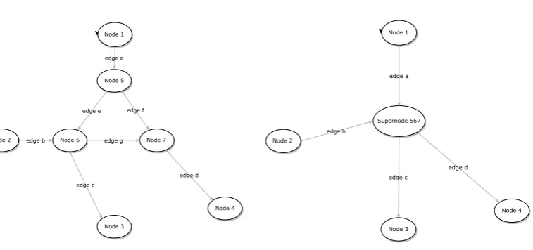
An illustration of the aggregation scheme is given in Figure 1. Nodes 5, 6 and 7 are aggregated into a supernode, and edges e,f and g are eliminated. The illustration can be considered part of a larger graph with other edges into and out of nodes 1,2,3 and 4, but no additional ones into or out of nodes 5,6 and 7. For components in order e,f,g, the matrixPAA in this case is given by

PAA=

 

0 0 Peg

0 0 0 0 0 0

edge b

edge c Node 1

edge e edge f

Node 5

Node 4 edge d Node 7 Node 6

Node 3

Node 2 edge g

edge a

edge b

edge c Node 1

Node 4 edge d

Supernode 567

Node 3 Node 2

edge a

Figure 1. Part of a graph and the result of aggregating nodes 5,6,7.

So

(I₋PAA)−1 =

 

1 0 Peg

0 1 0 0 0 1

 .

Equation (7) tells us how to update the waiting times on edges a,b and the transition probabilities from a, btoc, d.

The derivation of (7) is very similar to that of (3) and (4) for elimination of a group of nodes. In detail, the mean waiting time T0

e on edge eentering A for the new system

has to take into account the mean time to be spent in A before exiting. Thus T_e0 =

Te +P_u∈APeuT¯u, where ¯Tu is the mean time to first escape from A starting on u.

Now ¯Tu = Tu +P_v∈APuvT¯v, so the vector ¯TA = (I −PAA)

−1_T

A. Thus Te0 = Te+

PeA(I −PAA)−1TA. Similarly, Pef0 =Pef +Pu∈APeuP¯uf, where ¯Puf is the probability

that the first exit from A starting on edge u ∈ A is to edge f. This satisfies the equation ¯Puf = Puf +

P

v∈APuvP¯vf, so the vector ¯PAf = (I − PAA)−1PAf. Thus

P_ef0 =Pef+PeA(I−PAA)−1PAf. Note that (I−PAA) is invertible under the condition

thatAis leaky. IfAis not leaky there is no great point in computing when and to where one exits A. Note also that one can check thatP

fPef0 = 1 for the new system.

A downside of the aggregation scheme is that it may generate multiple edges between two nodes of the new system. For example, if there are edges from a node s not in A

to two nodes in A, the new system will have two edges froms toA. Similarly, if there are edges from two nodes in Ato a nodetnot in A, the new system will have two edges from Atot. One might hope that multiple edges could be aggregated into single edges. In general, however, this is not possible: if edges fi from a nodes to a nodetare to be

aggregated into a single edgef then for every edgeeintoswe must havePef =

P

iPefi, and for all edgeseinto sand gfrom twe must have P

iPefiPfig =PefPf g, but if there is more than one edge e into s this gives incompatible assignments to Pf g in general.

One solution is to aggregate s and t into one node, thereby not aggregating the edges

fi but eliminating them. This may produce other multiple edges elsewhere, however.

which nodes to aggregate. The scheme may also generate self-edges, but as with Wales’ second method, this is not necessarily a disadvantage.

Further aggregation can be performed, including putting super-nodes into clusters. They have no different status from the original nodes. One can also perform aggregation of disjoint subsets simultaneously, as the updates for edges entering or leaving disjoint sets of nodes do not interact.

At any stage of aggregation, the mean first passage time from an edgeeto a setB of edges not containingeis given by solving the usual system of equations

TeB =Te+

X

f /∈B

PefTf B

for the vector of mean first passage timesTeB.

One can think of the mean first passage time from a node s to a node t as being the occupation density at s resulting from injecting flux at rate 1 ats and taking out all matter arriving att. Thus it corresponds to the simplest case of a source and sink. We can tackle multiple sources and sinks, however, along the lines indicated in the Introduction.

The aggregation scheme can also be used to compute stationary probabilities. For example, the fraction on edge e is Te/Tee where Tee is the mean time of first return

to e, whose computation can be done via aggregation. Alternatively, the procedure of section 5 can be applied.

4. Aggregation of nodes as elimination of edges

It was mentioned in the previous section that the new aggregation method eliminates the edges between the nodes to be aggregated and that the derivation of (7) is very similar to that of (3,4). Actually, the new method is precisely elimination of nodes in the line-graph, using the version (3,4). This is made precise in the following proposition. It shall sometimes be convenient to include the weights explicitly by writing a quadruple

G= (V, E, T, P) to characterise our Markov flow.

Proposition 1. LetG= (V, E, T, P)be a Markov flow, and letX ⊂V. If one aggregates

X then one obtains a Markov flow on edges which naturally induces a Markov flow

Ga _{= (V}a_{, E}a_{, T}a_{, P}a_{) on the line-graph. Alternatively one may first naturally induce}

a Markov flow on the line-graph G0 = (V(G0), E(G0)) of G. Let B be the set of edges

in X. If one eliminates the collection of nodes in G0 _{induced by the edges B in G}

then one obtains a new Markov flow Ge _{= (V}e_{, E}e_{, T}e_{, P}e_{). The graphs G}a _{and G}e _are

isomorphic.

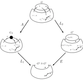
The proposition is illustrated in Figure 2.

First let us set up some notation. LetGX = (VX, EX) denote the weighted directed

graph resulting from aggregating X. Also, the standard procedure for constructing G0

ϕ−1 i (u)

ϕ−1 i (v)

G

X

V\X

GX

X

V\X L−₁1(u)

L−1 1 (v)

G′

L2(B)

E(G′)\L2(B) E−1 (u)

E−1 (v)

Ga_∼=Ge

u v

A

L

L

E

1

Figure 2. Illustration of Proposition 1

Proof of Proposition 1 . We will show that there is an isomorphismϕbetween (Va_{, E}a₎

and (Ve_{, E}e_{) as directed graphs without weights. Then we show ϕ preserves weights}

too. It is worth noting at this point that even ifGwere a multigraph (i.e. with possibly more than one directed edge from a node to another node), bothGa _andGe _{are merely}

graphs, and not multigraphs (this is a symptom of the fact that construction of both

Ga _{and G}e _{involves taking a line-graph, and not augmenting the set of edges after this}

action). So when showing our claimed isomorphism is indeed an isomorphism we know there can be at most a single edge between any two nodes.

First we find a bijection between E_\B and Va_{, as follows. Upon aggregation ofX}

in G the edges that are eliminated are exactly the edges in X, that is B. So there is a bijection A:E\B → EX (A for “aggregation”). Upon taking the line-graph of GX

we have a natural bijection (defined above) L1 :EX → Va, thus yielding the bijection

ϕ1=L1◦A we sought.

Similarly we construct a bijection between E _\ B and Ve_{. Let L}

2(B) denote the

collection of nodes inG0 induced by edgesB. There is a natural bijectionL2 :E\B →

V(G0)_\L2(B). Then as we eliminate exactly the set L2(B) of nodes in the line-graph

to form Ge _{there is trivially a bijection E :V(G}0_)\L

2(B)→ Ve (E for “elimination”)

and thus we find a bijectionϕ2 =E◦L2. Henceϕ=ϕ2◦ϕ−11 is a bijection Va→Ve.

Now we show that this bijection is indeed an isomorphism. Let u, v _∈ Va_{. We will}

show that (u, v)_∈Ea _{if and only if either (i) ϕ}−1

1 (u) is an edge entering X and ϕ

−1 1 (v)

destination node ofϕ−₁1(u) being the origin ofϕ−₁1(v). We shall also prove the analogous statement but taking instead u, v ∈Ve _{and replacing ϕ}

1 with ϕ2 in the above. These

two facts together implyϕis an isomorphism. Suppose (u, v)_∈Ea_{, then certainly the edgesL}−1

1 (u) andL

−1

1 (v) inEX lie end to end

with the destinationsof L−₁1(u) equalling the origin ofL−₁1(v). We consider two cases. First suppose thats6=X(remember, when we aggregate a collection of nodesXinGwe denote byXalso the supernode inGX). Then, upon undoing the aggregation, the nodes

ϕ−₁1(u) =A−1_◦L−1

1 (u) andϕ

−1

1 (v) =A−1◦L

−1

1 (v) still lie end to end. In the cases=X

then clearlyϕ−₁1(u) = A−1_◦L−1

1 (u) is an edge enteringX and ϕ

−1_{(v) =A}−1_◦L−1 1 (v)

is an edge leavingX since this is the only way that the destination ofL−₁1(u) and origin ofL−₁1(v) are both X.

Conversely supposeu, vare such that either (i) or (ii) holds. If we are in case (i) then the destination ofL−₁1(u) =A_◦ϕ−₁1(u) and the origin of L−₁1(v) =A_◦ϕ−₁1(v) are both

X. Since this means they lie end to end, upon taking the line-graph we recover that (u, v) _∈ Ea_{. If we are in case (ii) then again the destination of L}−1

1 (u) and the origin

ofL−₁1(v) must coincide (but not be equal to X, of course). Just as before, this implies that (u, v) _∈ Ea_{. Through highly similar arguments one can prove the corresponding}

statement originally taking instead nodes u, v ∈ Ee _{and replacing ϕ}

1 with ϕ2, thus

proving thatϕis an isomorphism. The final thing to check is thatTa

u =Tϕe(u)andPuva =Pϕe(u)ϕ(v) for allu, v∈Va. This

is almost trivial to see once one notices that when one naturally induces a Markov flow on edges of G, the mean waiting times and transition probabilities are just Te =TL2(e)

and Pef =PL2(e)L2(f) for alle, f ∈E. So finally, comparing equations (3,4) and (7) we

see the updates are identical.

The main conclusion to draw here is that to perform aggregation one can instead trans-fer to the line-graph, perform elimination and then undo the line-graph transformation. In a loose way one can think of this as meaning that aggregation and elimination are conjugate in the sense that LA=EL whereA, E, L represent performing aggregation, elimination, and moving to the line-graph respectively.

5. Relation to block LU decomposition

Another significant observation is that elimination schemes for Markov flows, whether on a graph or a line-graph, are closely related to block LU decomposition, as defined in [DHS, GW] for example. In particular, this connection makes clear how to keep track of quantities for parts for the system after they have been eliminated.

Let us review block LU decomposition, following [DHS]. To solve a linear system

Ax=b forx, split the components into two groups _{1,2_}chosen so thatA11 is easy to

invert. The idea is that we will eliminate the first group of components to reduce the problem to some linear system A0_x

2 = y2 but keep enough information to recover x1

too. First solve

forL21 (which is easy by hypothesis), and then write

(8)

A11 A12

A21 A22

=

I 0

L21 I

A11 A12

0 A0

with

A0=A22−L21A12.

To solveAx=bforx, first put

y2=b2−L21b1,

then solve

A0x2=y2

for x2 (this involves recursion because A0 will in general need simplifying in the same

way as we did with A), then solve

A11x1=b1−A12x2

forx1, which is easy because we supposedA11 is easy to invert.

Next, we apply block LU decomposition to the problem of computing the stationary probability distribution for a semi-Markov process. For non-eliminated nodes, this boils down to an application of Wales’ second method, but the block LU procedure shows how to compute it for eliminated nodes too. Suppose mean waiting time Ts at node

s _∈V and probability Pst for the next node t (allow Pss 6= 0). Stationary probability

π corresponds to πs = ρsTs with ρP = ρ and ρT = 1. We can solve for ρ by LU

decomposing the augmented matrix [I ₋P T] into parts for two disjoint node sets X

and Y where X ∪Y = V. X is assumed to be leaky (so I −PXX is invertible) and

I₋PXX is assumed to be easy to invert. The form of the desired LU decomposition is:

(9)

I₋PXX −PXY TX

−PY X I−PY Y TY

=

I 0

−LY X I

I₋PXX −PXY TX

0 I ₋P0

Y Y TY0

The block components are found by solving

LY X(I−PXX) =PY X

forLY X and then putting

P_{Y Y}0 =PY Y +LY XPXY

and

T_Y0 =TY +LY XTX.

To find ρ we solve

ρYPY Y0 =ρY, ρYTY0 = 1

forρY (recursively in general) and then extend by

ρX =ρYLY X.

At the end we put πs=ρsTs.

Lastly, we can use the same insight to compute mean first passage times to a subset B of nodes from all nodes outside B, not just non-eliminated ones. The vector of mean first passage times TB

a from nodes a ∈ A = Bc to a set of nodes B is the solution of

(I−PAA)T_AB =TA. Suppose we eliminate setX of nodes, disjoint from B, and we let

C be the complement ofX_∪B. Use the above LU decomposition, but just the part for

C inY. So solve

(I−P_CC0 )T_CB=T_C0

forTB

C (recursively in general). Then solve

(I₋PXX)TXB=TX +PXCTCB

forTB

X. One remaining issue to address is what happens if we eliminated some nodes of

B, but we leave that for later investigation.

6. Dynamics

Lastly, one might ask whether an aggregation scheme can be devised that keeps the dynamics, not just the steady state. Even in the Markov case, this can not be done with the above schemes because the dynamics of an N-state Markov chain has N −1 eigenvalues (counting multiplicity) so reduction of N must lose some of the dynamics. It can be done, however, if we replace the mean waiting time by the Laplace transform of the distribution of waiting times. This is because each Laplace component solves a steady state problem. The downside is that aggregation introduces rational functions of the Laplace transform variable s, whose degree increases as the number of nodes decreases.

7. Conclusion

A promising method for aggregation of Markov flows has been presented, which lends itself to iteration to produce a hierarchy.

After writing the paper we became aware of [Me] on stochastic complementation. Like our method, this is an adaptation of block LU decomposition to stochastic matrices. Meyer’s paper treats discrete time, whereas ours treats continuous time, but that is not a great difference. Instead of eliminating part of the system and working out how to keep track of properties for the eliminated part, he divides the system into two parts with equal status and some coupling between them. He treats only stationary distribution whereas we also treat mean first passage times, though again that is not a big extension. The main innovative feature of our paper that we think is useful is to perform the elimination on the line graph rather than the original graph.

A subsequent paper will report on tests of the method, including choices of hierarchy. For instance, we plan to compare with benchmark examples in [SW] on configurational transitions for Lennard-Jones clusters and a β-sheet peptide.

Competing interests

We have no competing interests.

Authors’ contributions

RM devised the aggregation scheme. JR showed that it is exactly an elimination scheme on the line-graph. We both worked out the application of block LU decomposition to computing stationary probabilities. JR wrote the proof that the aggregation scheme is an elimination scheme on the line-graph. RM wrote the rest with some polishing by JR. Both authors gave final approval for publication.

Acknowledgements

RM is grateful to David Wales for stimulating his interest in this topic. The ideas here were developed in response to Wales’ papers. The material of sections 1–3 was taught in a postgraduate module in Spring 2012 and RM is grateful to Erasmus Mundus masters students Aditya Challa and Yan Zhang for writing a report about them. The writing was carried out under a Royal Society Wolfson Research Merit Award for RM, followed by final year MMath project of JR. We are grateful to David Bindel for bringing stochastic complementation and nested dissection to our attention, and to a reviewer for references on lumping in chemical kinetics.

Funding statement

RM was supported by the University of Warwick and a Royal Society Wolfson Re-search Merit Award.

References

[Al] Allaire G, 2012, Introduction to homogenisation theory, in: Mathematical and numerical approaches for multi- scale problems, eds Canc`es E, Labb´e S, ch.1

[AS] Ando A, Simon HA, 1961, Aggregation of variables in dynamical systems, Econometrica 29, 111–138.

[A+] Auger P, de la Para RB, Poggiale JC, Sanchez E, Huu TN, 2008, Aggregation of variables and applications to population dynamics, in: Structured Population Models in Biology and Epidemiology, LNM 1936, Mathematical Biosciences Subseries. Edited by: Magal P, Ruan S. pp 209-263. Berlin: Springer

[B+] B´erenguier D, Chaouiya C, Monteiro PT, Naldi A, Remy E, Thieffry D, Tichit L. 2013, Dynamical modeling and analysis of large cellular regulatory networks. Chaos 23(2):025114. [CW] Carr JM, Wales DJ, 2008, Folding pathways and rates for the three-strandedβ-sheet peptide

Beta3s using discrete path sampling, J Phys Chem B 112, 8760–9

[CM] Catarino N, MacKay RS, 2005, Renormalization and quantum scaling of Frenkel-Kontorova models, J Stat Phys 121, 995–1014.

[CKMM] Cohen-Addad V, Kanade V, Mallmann-Trenn F, Mathieu C, 2017, Hierarchical Clustering: Objective Functions and Algorithms, arXiv: 1704.02147

[DRS] Davis TA, Rajamanickam S, Sid-Lakhdar WM, 2016, A survey of direct methods for sparse linear systems, Acta Num 383–566

[DHS] Demmel JW, Higham NJ, Schreiber RS, 1995, Stability of block LU factorization, Num Lin Alg Appl 2, 173–190

[DB] D¨orfler F, Bullo F, 2013, Kron reduction of graphs with applications to electrical networks, IEEE Trans Circuits Sys I 60, 150–163.

[EELRV] E W, Engquist B, Li X, Ren W, Vanden-Eijnden E, 2007, Heterogeneous multiscale methods: a review, Comm Comput Phys 2, 367–450.

[FH] Fortunato S, Hric D, 2016, Community detection in networks: a user guide, Phys Rpts 659, 1–44.

[FVH] Fr¨anti P, Virmajoki O, Hautam¨aki V, 2006, Fast agglomerative clustering using ak-nearest neighbour graph, IEEE Trans Pattern & Machine Intell 28, 1875–81.

[GW] Georgiev K, Wasniewski J, 2001, Recursive version of LU decomposition, in: Vulkov L, Was-niewski J, Yalamov P (eds), Lect Notes Comp Sci 1988 (Springer) 325–32

[GBDD] Grigori L, Boman EG, Donfack S, Davis TA, 2010, Hypergraph-based unsymmetric nested dissection ordering for sparse LU factorization, SIAM J Sci Comput 32, 3426–46

[Hu1] Hunter JJ, 2017, The computation of mean first passage times for Markov chains, arXiv 1701.07781

[Hu2] Hunter JJ, 2016, Accurate calculations of Stationary Distributions and Mean First Passage Times in Markov Renewal Processes and Markov Chains, Special Matrices 4, 151–175 [Il] Ille P, 1997, Indecomposable graphs, Discrete Math 173, 71–8

[KS] Kemeny JG, Snell JL, 1976, Finite Markov chains (Springer)

[LR] Li, G., Rabitz, H., 1989. A general analysis of exact lumping in chemical kinetics. Chem. Eng. Sci. 44, 14131430.

[LLJ] Lin, B., Leibovici, C.F., Jorgensen, S.B., 2008. Optimal component lumping: problem formu-lation and solution techniques. Comput. Chem. Eng. 32, 1167–72

[MBB] Machowski J, Bialek JW, Bumby JR, 2008, Power system dynamics (Wiley).

[M91] MacKay RS, 1991, Scaling exponents at the transition by breaking of analyticity for incom-mensurate structures, Physica D 50, 71–79

[M95] MacKay RS, 1995, The classical statistical mechanics of Frenkel-Kontorova models, J Stat Phys 80, 45–67

[M] MacKay RS, 2011, Hierarchical aggregation of complex systems, in: CRP2011 Position Papers,

http://lora.maths.warwick.ac.uk/groups/eccs sc/wiki/c8c73/CRP Forum 2011.html

(for EC FET-Proactive call on “Dynamics of multilevel complex systems”, session at ECCS11, Vienna).

[Me] Meyer CD, 1989, Stochastic complementation, uncoupling Markov chains, and the theory of nearly reducible systems, SIAM Rev 31, 240–272

[OZ] Owhadi H, Zhang L, 2007, Metric-based upscaling, Commun Pure Appl Math 60, 675–723. [POM] Porter MA, Onnela J-P, Mucha PJ, 2009, Communities in networks, Notice Am Math Soc 56,

1082-97, 1164-6.

[Saad] Saad Y, www-users.cs.umn.edu/∼saad/software

[SS] Sanders P, Schultes D, 2006, Engineering highway hierarchies, in: ESA 2006, Lect Notes in Computer Science 4168 (Springer) 804-816

[Si] Simon HA, 1962, The Architecture of Complexity, Proc Am Phil Soc 106, 467-482. [Sg] Sgurev V, 1993, Markov flows (Bulgarian Academy of Sciences, Sofia) (in Russian)

[Sh] Shell MS, 2016, Coarse-graining with the relative entropy, in: Advances in Chemical Physics, ends Rice SA, Dinner AR (Wiley) ch.5

[Sh1] Sheskin TJ, 1985, A Markov partitioning algorithm for computing steady state probabilities. Oper. Res. 33, 228-235

[Sh2] Sheskin TJ, 1995, Computing mean first passage times for a Markov chain, International Journal of Mathematical Education in Science and Technology, 26:5, 729-735

[St] Stewart WJ, 1994, Introduction to the numerical solution of Markov chains (Princeton) [Wa] Wagner AMG, 1998/9, Introduction to algebraic multigrid, Lecture notes, Heidelberg [W1] Wales DJ, 2006, Energy landscapes: calculating pathways and rates, Int Rev Phys Chem 25,

237-282.

[W2] Wales DJ, 2009, Calculating rate constants and committor probabilities for transition networks by graph transformation, J Chem Phys 130, 204111

[WK] Wei, J., Kuo, J.C., 1969. A lumping analysis in monomolecular reaction systems: analysis of the exactly lumpable system. Ind. Eng. Chem. Fundam. 8, 114123

Mathematics Institute and Centre for Complexity Science, University of Warwick, Coventry CV4 7AL, UK