warwick.ac.uk/lib-publications
Manuscript version: Working paper (or pre-print)
The version presented here is a Working Paper (or ‘pre-print’) that may be later published elsewhere.
Persistent WRAP URL:
http://wrap.warwick.ac.uk/132026
How to cite:
Please refer to the repository item page, detailed above, for the most recent bibliographic citation information. If a published version is known of, the repository item page linked to above, will contain details on accessing it.
Copyright and reuse:
The Warwick Research Archive Portal (WRAP) makes this work by researchers of the University of Warwick available open access under the following conditions.
Copyright © and all moral rights to the version of the paper presented here belong to the individual author(s) and/or other copyright owners. To the extent reasonable and practicable the material made available in WRAP has been checked for eligibility before being made available.
Copies of full items can be used for personal research or study, educational, or not-for-profit purposes without prior permission or charge. Provided that the authors, title and full
bibliographic details are credited, a hyperlink and/or URL is given for the original metadata page and the content is not changed in any way.
Publisher’s statement:
Please refer to the repository item page, publisher’s statement section, for further information.
Warwick Economics Research Papers
ISSN 2059-4283 (online)
ISSN 0083-7350 (print)
Secession with Natural Resources
Amrita Dhillon, Pramila Krishnan, Manasa Patnam and Carlo Perroni
(This paper also appears as CAGE Discussion paper 453)
Secession with Natural Resources
∗Amrita Dhillon† Pramila Krishnan‡ Manasa Patnam§ Carlo Perroni¶
December 2019
ABSTRACT
We look at the formation of new Indian states in 2001 to uncover the effects of political secession on the comparative economic performance of natural resource rich and natural resource poor areas. Re-source rich constituencies fared comparatively worse within new states that inherited a relatively larger proportion of natural resources. We argue that these patterns reflect how political reorganisation af-fected the quality of state governance of natural resources. We describe a model of collusion between state politicians and resource rent recipients that can account for the relationships we see in the data between natural resource abundance and post-breakup local outcomes.
KEYWORDS: Natural Resources and Economic Performance, Political Secession, Fiscal Federalism
JEL CLASSIFICATION: D72, H77, O13
SHORTTITLE: Secession with Natural Resources
∗We would like to thank seminar/conference participants at the Political Economy Workshop 2018, Helsinki, Paris School of Economics, Université Libre de Bruxelles, Queen Mary University of London, Kings College, London, University of Cam-bridge, London School of Economics,University of Oxford, European Development Network 2015, Oslo, Delhi School of Economics, Indian Statistical Institute, York University, University of Warwick, 3rd InsTED Workshop Indiana University, Econometric Society North American Summer meetings, for their comments. We would also like to thank Denis Cogneau, Stefan Dercon, Douglas Gollin, Eliana La Ferrara, Paolo Santos Monteiro, Kaivan Munshi, Rohini Pande, Andrew Pickering, Debraj Ray, Janne Tukiainen, and two anonymous reviewers for their comments on various versions of this paper. Financial support from the LABEX ECODEC (ANR-11-IDEX-0003/Labex Ecodec/ANR-11-LABX-0047) is gratefully acknowledged.
†Dept. of Political Economy, Kings College, London, and CAGE, University of Warwick. Email: [email protected]. ‡University of Oxford and CEPR, [email protected]
§CREST-ENSAE, [email protected]
1 INTRODUCTION
Does political secession yield economic dividends? Evidence on this question is mixed.1 Secessionist movements are often motivated by economic incentives; and in several cases these incentives relate to the ownership of natural resources (Collier and Hoeffler 2006).2 But some of the effects of political secession come from its effects on governance, effects that may be shaped by the re-allocation of nat-ural resources. Indeed, political secession provides a natnat-ural test-bed for investigating whether the widely-documented adverse influence of natural resources on economic performance (the “curse” of natural resources) flows through a political channel.
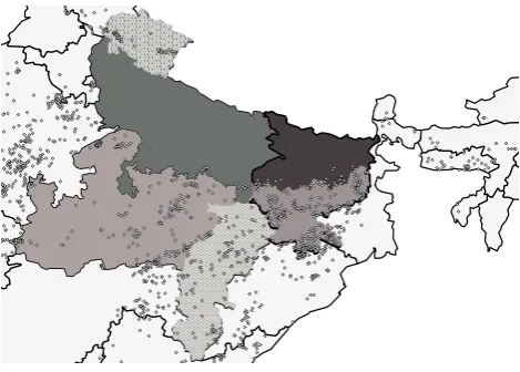
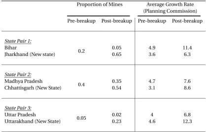
In this paper, we exploit the formation of three new Indian states in 2001 to examine how post-secession outcomes for local economies vary according to the local distribution of mineral deposits. A key feature of the 2001 Indian secession is that two of the original states contained a significant share of India’s natural resources, and these were concentrated within specific geographical areas. Figure 1 shows the states that were involved: the states that seceded are Jharkhand, Chhattisgarh and Uttarak-hand; the associated rump states are Bihar, Madhya Pradesh and Uttar Pradesh. Figure 2 illustrates the dramatic shift in control of mineral deposits from the original state to the new states. Table 1 gives a summary of the spatial distribution of natural resource rich (NRR) constituencies pre and post break up, in Columns 1 and 2. The Bihar-Jharkhand state pair witnessed a large change in the distribution of natural resources upon breakup, with Jharkhand (the new state) obtaining almost all of the min-eral deposits relative to Bihar. The breakup of Madhya Pradesh did mean that a substantial part of its natural resources accrued to the new state of Chhattisgarh, though Madhya Pradesh remains one of the states that are richer in natural resources. Finally, the Uttar Pradesh-Uttarakhand state pair saw a high proportion of mineral deposits go to Uttarakhand. The secession episode thus provides a quasi-natural experimental setting for examining how natural resource endowments are reflected in economic outcomes through political reorganisation.
Using a combined spatial discontinuity with difference-in-difference design, we examine the dif-ferential effects of the breakup on economic performance across new (seceding) and old (rump) states by examining the evolution of economic activity, proxied by luminosity, for 1,124 constituencies in the three pairs of states, comparing outcomes across the new state borders for 186 assembly constituen-cies (ACs) that are natural resource rich and for 938 ACs that are not, over the period 1992-2010. This allows us to study how seceding natural resource rich (NRR) constituencies perform relative to rump NRR units and how seceding natural resource poor (NRP) constituencies perform relative to rump NRP units.3 The borders of the assembly constituencies remained the same after secession making meaningful comparisons possible. Focusing on longitudinal, within-country comparisons allows us to circumvent some of the problems inherent in cross-country analyses.4
To identify the effect of state breakup on development outcomes, we make use of the geographic discontinuity at the boundaries of each pre-breakup state. We additionally exploit the time dimension of our data as a further source of identification. Essentially, we use the observedchangesin outcomes
1Rodríguez-Pose and Stermšek (2015), examine successive secession movements in the former Yugoslavia and find no
evidence of an independence premium. Rose (2006), on the other hand, finds no evidence that a larger size is beneficial. Theoretical analyses of the question (e.g. Boffa et al. 2016) have also pointed to a trade-off in decentralisation between the gains from policies that are better matched to local preferences and the potential loss of political accountability that can occur in smaller jurisdictions.
2E.g., the secession of South Sudan, rich in oil, from the rest of Sudan; or the case of Scotland, where the slogan “It’s
Scotland’s Oil” was used to promote the cause of independence. Sablik 2015 offers a useful summary.
3An assembly constituency is a state-level electoral unit which, under India’s first-pass-the post electoral system, elects
one member of the state legislative body.
4Cust and Poelhekke (2015) discuss these advantages and document other related studies on natural resources in a
Figure 1: Reorganisation of states in 2001
The figure shows the breakup of states in 2001. Areas shaded by dots represent newly created states; these are the states of Jharkhand, Chhattisgarh and Uttarakhand, which broke away from Bihar, Madhya Pradesh and Uttar Pradesh respectively. The map is representative of the political boundaries in 2001 (Administrative Atlas of India, Census of India, 2011).
Figure 2: Distribution of mineral deposits across the reorganised states
[image:5.595.181.416.517.685.2]Table 1: Endowment of natural resources and growth across states
Proportion of Mines Average Growth Rate (Planning Commission)
Pre-breakup Post-breakup Pre-breakup Post-breakup
State Pair 1:
Bihar
0.2 0.05 4.9 11.4
Jharkhand (New state) 0.65 3.6 6.3
State Pair 2:
Madhya Pradesh
0.4 0.35 4.7 7.6
Chhattisgarh (New State) 0.54 3.1 8.6
State Pair 3:
Uttar Pradesh
0.05 0.02 4 6.8
Uttarakhand (New State) 0.23 4.6 12.3
This table reports the level and change in the proportion of natural resource rich constituencies (i.e, those with mining deposits) after state reorganisation, as well as the level and change in growth rate (measured by gross state domestic prod-uct), for each state. Figures for the annual growth rate of each state were obtained from the Planning Commission of India’s figures for state-wise growth.
to difference outfixed, initial differences between units on either side of the border. Our identifying assumption is, therefore, that the other (initial) underlying discontinuities at the cutoff (for example, due to pre-defined administrative boundaries, like districting, or language differences) are not chang-ing over time, so that the differenced estimates should be unbiased for the local average treatment effect.
The results we obtain are striking. Specifically, NRR constituencies perform comparatively worse in the seceding (new) states; economic outcomes for NRP constituencies, on the other hand, are less affected by secession. Moreover, we find suggestive evidence of an interaction effect with natural re-source density at state level: NRR ACs in seceding states that inherit a higher proportion of NRR ACs perform worse relative to NRR ACs in the rump states. Our findings are supported at the aggregate level by figures from the Planning Commission (Table 1, columns 3 and 4), which show that although on average new states do better relative to rump states, post break up, we see heterogeneity in outcomes: areas in new states that end up with a much larger abundance of natural resources (Jharkhand) do worse than the rump state, while others perform better. The heterogeneity in outcomes at the local and state level is mirrored in changes in the distribution of natural resources across the newly-formed states. The heterogeneity in outcomes at the local and state level is mirrored in the distribution of natural resources across the newly-formed states. Following breakup, the proportion of ACs that are rich in mineral deposits is 65% in Jharkhand, up from 20% in the original, combined state (Table 1). The corresponding figures for Chhattisgarh and Uttarakhand are respectively 54% (up from 40%), and 23% (up from 5%). Thus, not only is the proportion of ACs that are natural resource rich higher for Jharkhand than it is for the other two newly-formed states, but Jharkhand is also the new state that experiences the largest natural endowment shock.5
A natural candidate explanation for this pattern is the change in state-level political institutions that followed from secession. And indeed our main finding of theinteractioneffect between natural resource abundance created by secession at the state level together with natural resource abundance at the assembly constituencies (AC) level is strongly suggestive of a channel flowing through a change in the political relationship between states and natural resource rich ACs following secession. In the case of India, this relationship is shaped by a number of features that are peculiar to the Indian context: (i) property rights to natural resources belong to states rather than to ACs; (ii) power is concentrated at the state level in terms of policing and public goods; (iii) royalty rates on minerals were very low in the period we consider;6(iv) there is a well-documented association between rent seeking, criminal activity and the abundance of natural resources (Vaishnav 2017; Aidt et al. 2011).
Building on this picture, Section 3 models the differential effects of secession on NRR and NRP districts as arising from a political bargain struck in NRR constituencies between state-level politi-cians and local rent recipients who control local votes and exchange them for natural resource rents. The greater is the proportion of NRR constituencies in the state, the greater is the state government’s comparative dependence on votes that are delivered by local-level patrons in return for rents, and the lower is political accountability in the state. State secession leads to a change in the proportion of NRR districts within a state and thus in the comparative importance of votes from NRR constituen-cies. As a result, states that inherit a comparatively large fraction of NRR districts can experience a loss of political accountability following secession, which in turn can lead to more intense rent grab-bing and worse economic outcomes in those areas. This is similar in spirit to the “preference dilution effect” described in the literature on lobbying, whereby more centralised decision making can reduce the power of lobbies to influence policies because of increased preference heterogeneity (e.g. de Melo et al. 1993). Our theoretical framework suggests that, when resource endowments are particularly high, they are more likely to lead to perverse outcomes.
The three instances of state breakup that we study translate into only six observed changes in the proportion of NRR districts within the new states by comparison with the original state. Neverthe-less, the patterns that we see in the data are in line with our interpretation that the effects we see come from the interplay of politics and natural resources. We see differential effects for NRR districts varying according to their political leanings. Further corroboration comes from investigating how the comparative performance of NRP and NRR districts varies with the election cycle: secession changes how the comparative performance of NRP and NRR districts vary over the cycle. These additional findings provides suggestive evidence that this performance gap is shaped by a political channel and that this channel is affected by political secession. It is also consistent with our interpretation of the effects of state breakup on the relationship between actors in NRR districts and state-level politicians. As we discuss later, these changes in performance between NRR and NRP areas are hard to reconcile with alternative explanations.
The remainder of the paper is organised as follows. Section 2 describes the institutional context. Section 3 presents a theoretical model that links political structure with the governance of natural resources. Section 4 presents the data used for analysis and lays out the identification strategy for estimating the effect of breakup. Sections 5 and 6 report the empirical results. Section 7 concludes.
discovered much later in the 1970s, following which Norway’s growth rate went down from 6.3% to 1.1%, measured over the period 1961 to 2016, while Sweden went from 5.7% to 3.2% over the same period (World Bank). More recent cases include the secession of South Sudan in 2011 with extensive oil resources but facing conflict and negative rates of growth (World Bank).
6Royalty rates here are not directly comparable to other international rates since they are based on weight rather than
2 THE INSTITUTIONAL CONTEXT
2.1 THE GOVERNANCE OF NATURAL RESOURCES ININDIA
India has a federal structure, with both national and state assemblies. Members of the twenty-nine state assemblies are elected in a first past-the-post system. The leader of the majority party or coalition is responsible for forming the state government. States have executive, fiscal and regulatory powers over a range of subjects that include education, health, infrastructure and law and order.
There is an overlap in authority between the federal government and state governments in the governance of natural resource extraction, with both exerting regulatory authority: major minerals such as coal and iron ore are regulated by the central government, while minor minerals are entirely under state control as laid down in the Mines and Minerals Development and Regulation (MMDR) Act of 1957. Royalty revenues accrue to state budgets, but rates are set by the central government, which controls rates on output as well as any “dead rent” that accrues in the absence of extraction, and also decides on environmental clearances for mining. Property rights to land reside in the states, which are the legal owners of all major mineral resources (except uranium), and claim all royalties. The main power of the states derives from the legal authority to grant licenses. However, until recently, there was no requirement for the royalties and returns from mining to accrue to local areas and the entire proceeds accrue to the state budget.7 There are thus three players involved in royalty on minerals: the Central Government which fixes the royalty rate, mode and frequency of revision; the State Gov-ernment, which collects and appropriates royalty; and the lessee who might be in either the public or private sector and who pays the royalty according to the rates and terms fixed by the centre to the State.
The split of authority between federal and state agencies with respect to the governance of natural resources means that the effects of policy decisions at each level are not fully internalised. The roy-alty rates set by the central government are widely seen as being inefficiently low,8lowering incentives for states to allocate extraction rights to efficient operators and to police illegal mining, since royalties from mining contribute so little to their budgets: royalty revenues in these states, as a percentage of to-tal revenue, averaged to two percent in 2009, while the mining sector’s share of state domestic product is an average of 10-11 percent for Jharkhand and Chhattisgarh over the period 2004-2011 (Chakraborty and Garg 2015). Low royalty rates also mean that there is little scope for state politicians to translate their control rights over natural resources directly into “political rents” for themselves (e.g. by using royalty revenues to finance popular public projects or transfers), which in turn means that in order to do so they must use indirect channels to do so (e.g. using allocating natural resource rights to buttress political support). The fact that the authority for policing resides with the state governments while the federal government decides on which areas can host mining activity produces incentives to evade en-vironmental regulations by operating outside the areas given clearance by the federal government. All of this has led to conflict between Centre and State about the weak policing and monitoring by state governments.9 Given this institutional context, the politics of resource extraction in India takes on a different flavour from that seen in some other federal states. Natural resource rents are controlled by local operators but power resides at the state level- in particular, as mentioned before, the pro-vision of education, health, law and order and rural electrification is firmly under state control. This
7The recent Mines and Minerals (Development and Regulation) Amendment Ordinance, 2015 provides for the creation of
a District Mineral Foundation (DMF) and a National Mineral Exploration Trust (NMET), funded by a percentage of royalties paid by lessees and in principle, affording some re-distribution to local communities.
8It is difficult to compare royalty rates with international rates as the latter are mostly ad valorem while in India royalty
rates have been based on weight until recently. A switch to ad valorem rates in 2009 increased revenues on iron ore ten times (Vanden Eynde 2015).
institutional setting creates the conditions for state-level politicians and local leaders to strike a politi-cal bargain where they trade “subterranean rents” for loyalty and votes.10This link between state-level politicians and local rent-seekers is incontrovertible: the political scientist Milan Vaishnav documents this in detail in his account of the criminality of politicians (Vaishnav 2017). He argues that the rising cost of elections and a shadowy election financing system where parties and candidates under-report collections and expenses means that parties prefer “self-financing candidates who do not represent a drain on the finite party coffers but instead contribute ‘rents’ to the party”; and tells of how, in the state of Jharkhand, the minister in charge of mines (Koda) once disposed of 48 cases in one hour. Indeed, the corruption is so institutionalised that one of the chairmen of Coal India in West Bengal says that ministers would fix monthly payment targets with senior executives of Coal India and this was one of the main sources of funding for political parties. According to some reports almost 15-20% of mining revenues are creamed off every month (see Spectator Magazine, 2009).
At the local level, natural resource rents give rise to widely documented forms of “rent grabbing”, both legal and illegal. Legalised rent grabbing consists of comparatively less efficient but politically connected producers successfully securing resource extraction rights.11 Illegal rent grabbing mainly consists of illegal mining. Collusion of local “rent grabbing entrepreneurs” with corrupt state-level politicians is required to sustain either form of rent grabbing.12Not only do states grant licenses and leases, but the Mines and Minerals Development and Regulation Act 1957 empowers state and central government officers to enter and inspect any mine at any time. Thus, illegally extracting minerals from these areas requires a degree of endorsement from the state – e.g. the police turning a blind eye to illegal activity, or favouritism in allocating leases. These rent grabbing activities generate visible economic costs for local economies, ranging from losses in production efficiency and a deterioration of law and order, to environmental degradation, displacement of local residents, disruption of local infrastructure — all leading to a crowding out of other economic activities (Baland and Francois 2000, Mehlum et al. 2006).13
The lack of response by state-level governments to such rent-grabbing, despite the fact that they have jurisdiction over all mining matters, suggests that there is a bargain being struck, in NRR ACs, between state-level politicians and the local-level political entrepreneurs/patrons, with payments for concessions made by politicians in relation to natural resource rents – directly, through the allocation of mining rights, and indirectly, through lax controls on how those rights are managed at the local level – taking the form of either bribes or increased political support from local constituencies. The
10Indeed, many times the local rent grabbing entrepreneurs become politicians themselves. Asher and Novosad (2016)
documents how local mineral rent shocks cause both adverse selection and worse behaviour of politicians in office. They describe how local politicians have direct control over mining operations from which they derive rents. Aidt et al. (2011) shows how stiff competition between parties in India creates an inherent advantage for criminal politicians who can buy votes or intimidate voters.
11The allocation process itself, however, is often fraught with irregularities: in 2014 the Supreme court ruled that more
than 214 out of 218 coal licences awarded by governments between 1993-2010 were illegal (see BBC News).
12The Shah Commission Report available athttp://www.mines.nic.inprovides an ongoing saga of the types of
ex-cesses that go on in mining areas.
13As a specific example, take the case of coal: “It is a murky subculture that entwines the coal mafia, police, poor villagers,
latter relies on local rent recipients being able, through either persuasion or coercion of local voters, to deliver a certain volume of votes to whichever candidate or party they choose.
Vote buying is pervasive in India, not only in NRR constituencies (see, e.g., Mitra et al. 2017); and it often involves handing out gifts or money prior to elections. Nevertheless, there are reasons to expect that this exchange of votes for favours to happen comparatively more in NRR ACs. This is because the state-level government controls the allocation of rights for the exploitation of natural resources as well as the enforcement of exploitation rights, but, as discussed earlier, due to the low royalty rates that are set by the federal government, the implications of these decisions for state-level revenues are negligible. State-level politicians thus have control over something that is very valuable to local operators but involves little economic opportunity cost for state budgets, making it a natural currency to be spent in a votes-for-favours transaction. Natural-resource poor (NRP) constituencies lack such currency.14
A symptom of the high prevalence of patronage politics in NRR areas is the higher likelihood of criminal politicians being elected in mineral rich constituencies. Table 10 shows that, in a sample of 179 Parliamentary Constituencies (electing federal level MPs), the likelihood of a politician with a criminal record being elected is increasing in the density of mines in that constituency (the coefficient from a simple OLS specification is positive and significant at the 5% level). There is also evidence, as shown in Table 10, that vote buying and electoral fraud takes place relatively more in the mineral rich areas: using survey responses from the State Election Survey for Jharkhand in 2005, which posed ques-tions to individual voters about percepques-tions of voting malpractices, and running a logit specification of perceived voting malpractice within a district against the number of mines within that district, in-cluding district fixed effects and controls for household characteristics, gives a coefficient of 0.28 that is significant at the 1% level.
2.2 EXOGENEITY OFBORDERS AND THETIMING OFSTATEBREAKUP
Tillin (2013) explores how the breakup of existing states in 2001 came about. She suggests four possi-ble explanations. The first explanation proffered is that of distinct cultural identities in the breakaway areas that have consistently made demands for secession, demands that have progressively gained prominence since 1947. The basis on which state borders were originally drawn by the State Reorgan-isation Act of 1956 was along linguistic boundaries, but this criterion tended to ignore other ethnic and social boundaries, leading to large tribal populations in some states seeing themselves as ethni-cally distinct and socially neglected. It should be noted, however, that the sharp distinctions along ethnic, social and linguistic lines, in pre-independence have been reduced in time, since migration and changing demographics have meant more homogeneity particularly along existing sub-regional or district borders – this point is explored in further detail below when we examine the balancing of characteristics along the border between states (see Table 2). Furthermore, not all these demands were centred around statehood, but they did involve claims for more local representation and local management of natural resources, both mines and forestries.15Second, and tied closely to our expla-nation here, Tillin suggests that natural resources were a factor: private interests might have consid-ered it easier to increase resource extraction and intensify production in a smaller jurisdiction, which
14This can be viewed as an extreme case of a more general scenario where vote trading can take place in all constituencies
but comparatively more so in natural-resource rich ones.
15Tillin (2013) writes “All three of the regions that became states in 2000 saw the emergence of distinctive types of social
she terms “extension of capitalist interests”.16 The third explanation relates to the changing federal election context since 1989, when the leading coalition partner, the Bharatiya Janata Party (BJP), first favoured granting statehood to boost their popularity in the areas concerned. This is plausible but as we explain below, a decade later all political parties had reached a consensus on agreeing secession in these states (Kumar 2010). A final explanation is that the sheer size of the old states made them diffi-cult to govern and that the breakup was attractive to the central government because it meant better governance and more ease of administration – as well as an acknowledgement of local identities.
The list of explanations Tillin (2013) offers for the 2001 breakup flags two potential difficulties in looking at secession as a true natural experiment. The first relates to how borders between the rump state and the breakaway state were determined. This turns out not to be an issue at all because the boundaries of these three new entities have never been in dispute; the areas comprising the new states were separate entities before independence from British rule in 1947. For instance, Sharma (1976) dis-cusses a memorandum to the State reorganisation commission in 1955 asking for a separate state of Jharkhand, naming the six districts in Bihar that were eventually separated from Bihar in 2000 (Haz-aribagh, Ranchi, Palamu, Singhbhum, Santhal Parganas and Dhanbad, then Manbhum).17 The Ut-tarakhand Kranti Dal, the regional party formed in 1979 for a separate hill state was determined to unite the eight hill districts in a separate entity. The borders of Uttarakhand were thus determined by the borders of the eight hill districts that maintained their separate identity on the basis of geography and cultural distinctiveness; again, these borders were not in dispute. The borders of Chhattisgarh comprised the eighteen districts where Chhattisgarhi was spoken, and, again, these district borders have remained the same since independence.18 However, a key challenge for identification is that de-spite the fact that the demarcation was determined in the past, differences across the borders might have evolved over time; this is examined further in Table 2 and in Section 5.1.
The second potential difficulty pertains to the timing of the breakup. This timing was determined by the success of the BJP at the National elections in 1998. The BJP had led a minority government in 1996 and had promised to grant statehood to the three new states if it was returned to power. It was returned again at the head of a coalition government, but by this time there was a general consensus both at national and state levels: the other leading party of the Congress supported the change, as did the state assemblies of the original states before breakup. While there might have been a initial spurt of political activity by the BJP,19 by this time there was little political opposition anywhere to the demands for statehood. In fact, these demands had grown less vociferous since the early 1990s because it was clear that all the major parties were in accord. Part of this unanimity lay in the fact that all three new states lie well within the external boundaries of India and thus posed little threat to the Union of India, and, equally important, it was clear that there was no political gain to any of the parties in opposing secession. It might be thought that the timing of breakup was related to particular advantages of the party in power at the Centre; however, given the consensus across parties and the
16Tillin (2013) summarises the views, both pre and post breakup, of Tata Steel, the major investor in Jharkhand, and that
of other industrialists. Tata Steel was happier with a larger state where “politicians were farther away in Bihar” and less likely to meddle, while others favoured a smaller state where they hoped there would be better law and order and less corruption. However, seven years after secession, things were perhaps even worse in the new state according to them. In brief, there were clearly mixed views and, far from the urge to expand resource extraction, issues of infrastructure, electricity provision and law and order loomed large in favouring breakup and evaluating its success.
17It was the case that the borders were formally decided so as to include the districts that consisted of ‘Scheduled Areas’ as
defined in the Constitution, which in turn may have followed the Simon commission of 1930 that defined certain ‘partially excluded areas’. The list of scheduled areas (which are still mentioned as part of the old states) is available at the Ministry of Tribal affairs website here http://tribal.nic.in/Content/StatewiseListofScheduleAreasProfiles.aspx.
18Since 2012 these borders have been redrawn to give nine new districts.
19The BJP and its previous incarnation, the Bharatiya Jan Sangh had always opposed any state breakup until the 1990s,
fact that state assemblies pre breakup gave their willing assent to the breakup without much dissent, this also turns out to be a non-issue (Kumar 2010).
Finally, given that we concentrate on the role of resources, it should be emphasised that the prices of minerals played little part in the timing: mineral prices worldwide see a surge only after 2004, four years after breakup. In summary, neither the borders of the states nor the timing of breakup can be traced to any particular economic or political advantage for the breakaway states.
2.3 POLITICALREORGANISATION ANDNATURALRESOURCES
In our empirical analysis, we ask how the relative economic performance of natural resource rich and natural resource poor areas was affected by secession. Unlike in the Brazilian case studied by Brollo et al. (2013) and by Caselli and Michaels (2013), state breakup in the Indian case could not have pro-duced windfall revenues at the local level that could have directly encouraged direct appropriation of rents.20 As we have discussed in Section 2, the political bargain between local and state level leaders might be mediated through bribes or votes. In the Indian case, however, there is no clear reason to expect bribery incentives to be much affected by secession, given that state breakup does not change the economic value of mining concessions and that the influence of state politicians on the allocation of rents remains unchanged.
On the other hand, political reorganisation might directly affect incentives to exchange natural re-source rents for local political support. A direct, mechanical effect of secession is a change in the struc-ture of political competition within states: each new state feastruc-tures fewer districts, each accounting for a larger share of the total votes. Then, if control over natural resources is used by state politicians as a means of securing political support in relevant districts, it is plausible that secession, by changing the relative political weight of NRR constituencies within the new states, would change the calculation of the political costs and benefits involved. And indeed, if we look at how secession has affected the com-parative density of natural resource districts across states, we see that the change in some cases has been dramatic: in the case of Bihar, for example, about 65% of all districts in the newly formed state of Jharkhand are natural resource rich, whereas the corresponding proportion pre-breakup was 20% (see Column 2, Table 1). In contrast, the state pair 3 (Uttar Pradesh and Uttarakhand) begins with a very small endowment of resources and while the split benefited the new state, it should be emphasised that a larger share of a small endowment did not benefit it greatly.
We formalise this idea in the next section.
3 POLITICALSECESSION, NATURALRESOURCES ANDVOTE TRADING
This section presents a stylised theoretical political-economy framework that derives predictions on how the changes in the concentration of natural resources brought about by secession can translate into changes in economic outcomes at the local level. The key idea underlying our modelling exercise is that the adverse effects of the political influence exerted by special interest groups grows stronger the smaller is the proportion of competing interests that might act to mitigate them.
The specific mechanism we model relates to an electoral accountability channel that operates at the state level, which arises from a bargaining game in NRR ACs involving vote sellers/patrons at the local level and vote buyers or parties at the state level (above and beyond the kind of vote buying
20Anecdotal evidence suggests that most corruption takes place at the stage of the allocation of licences, and
that might occur in any constituency independently of its natural resource endowments). The more valuable the votes are, the higher will be the concessions (the “price” paid for votes) to local level intermediaries. These concessions generate negative economic spillovers on the rest of the economy, which erode political support in the electorate, translating into political costs that must be balanced against the political gains that directly come from securing votes through patronage politics in the NRR ACs. State secession changes the distribution of NRR and NRP ACs within the newly formed states and thus alters the political trade-offs involved in vote buying, which in turn affects economic outcomes in NRR and NRP ACs.
We begin our discussion by presenting a single-state model of vote selling in political equilibrium and then extend it to characterise effects of secession.
3.1 VOTES FORSALE ANDNATURALRESOURCEDENSITY
Policy Preferences
Consider first a single state with a continuum of mass one of constituencies with populations of iden-tical size. A fractionq∈(0, 1)of all constituencies are natural resource rich (NRR) constituencies; the remaining fraction, 1−q, of constituencies are natural resource poor (NRP) and have no natural re-sources.
Each voter in each constituency has an ex-ante ideal point,i, in ideology/policy space[−1/2, 1/2]≡
I, withibeing uniformly distributed over the supportIin each constituency. A voter’s utility is quadrat-ically decreasing in the distance between her ideal policy,i, and the actual policy,i0: the payoff levels
a voteri obtains from policyi0is−(i−i0)2.
Two parties,L(the incumbent) andR(the challenger), compete in state-level elections. The win-ning party, j ∈ {L,R}, obtains political rents,W, which we assume to be unity without loss of gener-ality. The incumbent party thus aims at maximising expected political rents,PjWW =PjW, wherePjW
is the probability of party jwinning.
PartyLhas an exogenously specified platform located at−1/2 in ideology space, while partyRhas an exogenously specified platform located at 1/2. The payoff levels a voteriobtains ifLandRwin the election are thus respectivelyUiL=−(−1/2−i)2, andUiR =−(1/2−i)2, with the median ideology voter (i=0) being indifferent between the two parties. Additionally, there is a stochastic ideology shock,s, the same in all constituencies and uniformly distributed in[−1/2, 1/2], that shifts the ex-post ideology of voteritoi+s.21
Voters vote sincerely. For a given ideology shock,s, the shares of votes that are cast respectively for L andR are therefore equal to 1/2−s and 1/2+s; and so, in the absence of any vote trading, the probability of party L party winning coincides with the probability ofs being negative and the probability of partyR winning is the probability ofs being positive, both of which are equal to 1/2, given the assumed distribution of ideology shocks.22
21This incumbency related shock could be thought of, for example, as being linked to a common but unpredictable
as-sessment by voters of the incumbent’s performance while in office.sis a shock in favour of theRparty.
22We can assume that ifs=0 each of the two parties wins with equal probability; but since this is a measure zero event, it
The Price of Votes
In each NRR constituency, a local leader controls, through intimidation or persuasion, a fraction,v∈
(0, 1/2), of the total votes.23 (In Appendix B we discuss an extension in which there is a continuous distribution of natural resources across jurisdictions and where the proportion,q, of ACs where vote sales take place is endogenised on the basis of an economic calculation linking the value of natural resource rents with the cost of procuring votes.) The given tranche of votes,v, can only be delivered to a single party for a price,x. This price is a payment in kind consisting of targeted, natural resource related concessions that translate into rents for the sellers, such as, for example, granting exploitation rights, as well as relaxing restrictions and policing of abuses by those exploiting the natural resources illegally. The net economic value of these concessions to the sellers isz x (z >0). The price can be delivered to the seller only if the vote buyer wins the election: the seller’s expected payoff if votes are sold to party jfor a pricexis thereforePjWz x.
The rent grabbing activities associated with the payment generate a loss ofλx for those voters in the constituency who do not partake in them, as well as negative spillovers ofρx for voters in other constituencies. What we have in mind here are all the negative effects from unregulated mining – such as environmental degradation, underground coal fires that can interfere with other economic activities, intimidation by criminal gangs that enable rent extraction (Asher and Novosad 2016) – as well as the economic costs associated with extraction rights being allocated to less efficient operators or granted on deposits that should not be exploited on the basis of an economic calculation of social costs and benefits.24
Because of these adverse effects, the favours that are delivered in exchange for votes entail a po-litical opportunity cost for the buyer: since the losses associated with the exchange only occur upon delivery of the promised payment if the party that buys the votes is elected, they have the same effect as that of an ideology shift of corresponding magnitude amongst independent voters against the party that buys the votes. Specifically, suppose that all the votes that are available for sale in all constituen-cies are purchased by a single party, and that the transaction can be observed by voters;25independent voters in NRR constituencies would then anticipate an overall loss(λ+ρq)x from a win by that party, whereas the prospective loss for for voters in NRP constituencies isρq x.
The buyer, in its calculation, must balance off this loss of political support amongst independent voters against the electoral advantage of being able to secure a fraction of the votes directly through vote buying. In NRR constituencies the political cost arising from the promised delivery of the pay-ment is offset by the political gain from buying votes, but in NRP constituencies it is not. Because of this asymmetry, an increase in the proportion,q, of NRR constituencies makes vote buying more attractive, raising the equilibrium price of the votes that are available for sale:
Proposition 1: Consider the a single (collusive) vote seller making a take-it-or-leave-it offer to a single buyer. The unique payoff maximising price for the seller isx˜ = v
λ(1−v) +ρ(1−q v). This price is de-creasing inρand increasing in q , and its elasticity with respect to changes in q is also increasing in q . The corresponding equilibrium values of PLW are also decreasing inρand increasing in q .
23For accounts of the extent to which local leaders exert control upon the votes of local populations, see Rao (1983) and
Singh and Harriss-White (2019).
24For example, blasting and drilling around the coal mines lead to water aquifers drying up, air and noise pollution leading
to a shortage of clean drinking water and water borne diseases to increase, loss of forest reserves, loss of agricultural land, disruption of economic activity by Maoist insurgents (Chauhan 2010). These effects would not be limited only to mining regions but would spill over to neighbouring NRP ACs – particularly SO2 emissions, pollution of surface water, spillovers from criminal activities and insurgency.
(The proof is in Appendix B.)
Allowing for multiple buyers or sellers does not change conclusions. The results of Proposition 1 carry over to a scenario where neither party has all the bargaining power – e.g., under sequential bargaining with alternating offers (Rubinstein 1982). Both extensions are discussed in Appendix B.
An increase in the density of natural resources, via a political channel, raisesx and thus lowers economic performance (welfare) in NRR constituencies (for individuals other than the vote sellers), as well as in NRP constituencies, albeit to a lesser extent. The intuition for this result is as follows. In its choice of x, the incumbent party balances the net gain in vote share from raising x in NRR constituencies with the net loss in NRP constituencies. As the proportion of NRR constituencies (q) becomes larger – and the proportion of NRP constituencies (1−q) becomes smaller – the positive vote gains from vote buying in NRR constituencies increasingly come to dominate the political “dilution” effect that comes from the purely negative political spillovers in NRP constituencies, and so the net political value of vote buying (and hence the maximum price that can be paid for it) increases.
Proposition 1 also implies that the dilution effect fades progressively faster asqincreases: intu-itively, the strength of the diluting influence of NRP constituencies is related to the ratio (1−q)/q, which decreases withq at at an increasing rate (in absolute value). As a result, the adverse effects of an increase in the proportion of NRR ACs become progressively larger.
3.2 EFFECTS OFSTATEBREAKUP
State breakup can produce a change in the proportion of NRR districts within the new states relative to the original state. The predictions we have derived in the previous section for a single-state scenario thus translate into predictions on the effects of state breakup on governance outcomes – predictions that in principle could be tested empirically in longitudinal evidence on pre- and post-secession out-comes.
Consider a unified state,U, with a unit mass of constituencies, a fractionqU of which are NRR con-stituencies; and suppose that the unified state breaks up into two new equally-sized states,AandB, each with a mass of 1/2 constituencies and proportionsqAandqBof NRR constituencies. Then, focus-ing only on the component of utility that depends onx, welfare for a citizeni in a NRP constituency in stateH∈ {A,B}can be expressed as
UHN R P =−ρqHxH+γq−Hx−H
2 , H ∈ {A,B}; (1)
while that for the citizen in a NRR constituency is
UHN R R=UHN R P −λxH, H ∈ {A,B}, (2)
whereγ <1 reflects a reduction in transboundary spillovers coming from the separation of state insti-tutions, and(qA+qB)/2=qU.26
Votes inH only affect xH, and so only the terms that involve xH in (1) and (2) are relevant for characterising voting choices inH. In turn,xHdepends onqHvia the equilibrium condition described in Proposition 1.
We are then in a position to draw conclusions concerning how secession affects economic perfor-mance via the political channel described in 3.1 (i.e. abstracting for the time being from effects directly associated with the redistribution of revenues from natural resources):
26We abstract from any idiosyncratic component of utility stemming both from ideology and from other factors that do
Proposition 2: The ratio UAN R P/UBN R P and UAN R R/UAN R P are both increasing in qA/qB. As levels of
utility are normalised in the model to be negative, this means that, following secession:
(i) comparing across states, UN R P
A is smaller, relative to UBN R P, the larger is qArelative to qB;
(ii) within state A, UAN R Ris smaller, relative to UAN R R, the larger is qArelative to qB.
(The proof is in Appendix B.)
This result follows immediately from our analysis of a single-state scenario. A higher proportion of natural resource rich districts within a state worsens the quality of governance, and hence economic performance, in that state. To the extent that spillover effects across states are weaker than those within states, this implies that, when we consider only those effects of natural resources that flow through a governance channel, an unequal allocation of NRR districts following secession penalises the state that receives the larger share (prediction 2.(i)); and, more specifically, worsens the compara-tive economic performance of NRR areas relacompara-tive to that of NRP areas (prediction 2.(ii)). As explained in the introduction, this is similar to a “preference dilution effect” whereby more centralised decision making reduces the power of lobbies to influence policies. In our particular context, secession has similar effects to decentralisation where the power of local rent seeking lobbies in NRR ACs increases relative to other interest groups when their relative weight increases.
Proposition 2 isolates those effects of secession that flow through the political channel we have described in 2.1, but secession also produces effects that flow directly through the redistribution of natural resource revenues. These effect relate to the change in the natural resource tax base base,
(qA−qU)r, wherer is total income from natural resources in a representative NRR ACs. An increase inqrelative to its pre-secession level produces an increase in the tax base (relative to the size of the new state), which may either translate into more provision of public goods, either state-wide or at the NRR AC level, or, alternatively, into a lower level of taxation holding the level of public goods provision constant, leaving more disposable income within NRR ACs.27 Through this effect, an increase inq
can potentially raise economic performance in the new state, and, more specifically, in NRR ACs; and indeed, as discussed, the reallocation of revenues from natural resources is often a primary motivation for secession demands.
Proposition 1 says that the effects of an increase inqonxincrease withq– as the diluting influence of the remaining fraction, 1−q, of NRP ACs becomes progressively smaller, the elasticity ofx with respect to changes in 1 becomes larges, (i.e. the cost associated with a higherq is convex inq). And so, if the post-secession level ofqAis large enough, the adverse governance effects of an increase in
qA, as described by Proposition 2, are more likely to dominate any other positive effects (such as those effects that are associated with an increase in the tax base, which is linear inq), leading to NRR ACs doing comparatively worse than NRP ACs in stateApost secession (result 2.(ii)):
Proposition 3: Political secession is more likely to lead to a deterioration in the comparative economic performance of NRR ACs relative to that of NRP ACs of the breakaway state the larger is the density of natural resources in the breakaway state post secession.
The predictions of the theory in relation to the effects of political secession can be summarised as follows:
27There may be other effects of the breakup on economic performance that are independent of the endowment of natural
• an increase in the proportion of NRR (q) in a breakaway state following secession will weaken the diluting effect that NRP areas exert on the political influence of natural resource rents recipients in NRR areas and lower the quality of governance and thus economic performance;
• this effect is more likely to dominate other positive effects associated with increased ownership of natural resources in the breakaway state (and result in a comparative worsening in the eco-nomic performance of NRR ACs relative to that of NRP ACs) the larger isqin the breakaway state post secession.
4 DATA
To study how differences in local outcomes (assembly constituency level) relate to natural resources we rely on two main data sources.
First, we rely on luminosity data to proxy for the evolution of economic activity (Henderson et al. 2011; Chen and Nordhaus 2011; Kulkarni et al. 2011; Alesina et al. 2016), over the period 1992-2010, thus covering the pre-breakup period 1992-2001, and the post-breakup period 2002-2010.28The data consist of imaging of stable lights obtained as a global annual cloud free composite where the ephemeral lights from fires and other sources are removed and the data are averaged and quantified in six bits, which in turn might result in saturation for urban settings but does mean that dimmer lights in rural settings are captured. Each grid (one sq. km) is assigned a digital number (DN) ranging from 0 to 63 and luminosity is measured as the DN3/2. Luminosity is thus obtained as a sum of lights over the gridded area which in our case is defined as the Assembly Constituency (AC), using GIS data on the administrative boundaries of states and ACs.29
There are three main reasons why we rely on luminosity data. The first is that panel data on house-holds, by assembly constituencies30that could capture the evolution of incomes or consumption pre and post breakup does not exist. The second reason is that, despite the measurement difficulties in-herent in the use of such a proxy, there is convincing evidence to suggest that luminosity is strongly cor-related with standard socio-economic outcomes. We offer corroborative evidence for this by looking at the relationship between luminosity and these measures; in brief, we use data on income, wealth and education from the National Election Survey in the year 2004, which surveys voters at the constituency level to examine the correlation of standard economic indicators with luminosity. The correlation with wealth is about 0.6, while that with income and education lies between 0.4 and 0.45.31 This relation-ship also holds at the more aggregate level of the district: Chaturvedi et al. (2011) and Bhandari and Roychowdhury (2011) examine this correlation at the district level in India and find similar effects. We restrict our analysis to the years 1992-2010 because constituency borders have since been re-drawn.32 The third (and most important) reason for relying on luminosity evidence is that our identification
28The night time image data is obtained from the Defense Meteorological Satellite Program Operational Linescan System
(DMS P-OLS). The DMSP satellites collect a complete set of earth images twice a day at a nominal resolution of 0.56 km, smoothed to blocks of 2.8 km (30 arc-seconds). The data, in 30 arc-second resolution (1km grid interval), covers 180◦West to 180◦East longitude and 65◦North to 65◦South latitude.
29We are grateful to Sam Asher and Paul Novosad who provided the geographic data necessary for matching electoral
constituencies to mineral deposits which in turn comes from the MLInfomap Pollmap dataset, which contains digitised GIS data based on maps published by the Election Commission of India.
30Districts are at a higher level of aggregation than assembly constituencies.
31The National Election Survey collects information from voters in each parliamentary constituency. To obtain the
corre-lations, we aggregate the night-time lights data to the parliamentary constituency level.
32The boundaries for constituencies were fixed in 1976 but new boundaries based on the 2001 census figures were meant
strategy focuses onchangesin outcomes rather than levels. This means that sources of persistent het-erogeneity across ACs in the relationship between luminosity levels and levels of economic activity are not a concern.
To corroborate our measure of night-time lights, we use data from two waves (1992 and 2004) of the India Human Development Survey (IHDS). Finally we also use data from the Census of India, state election results (obtained from the Election Commission of India) and state electricity prices (obtained from India Stat) to support our identification strategy, described in the next subsection. Appendix A provides further details on these data sources.
The second type of data we use are data on the location, type and size of mineral deposits from the Mineral Atlas of India (Geological Survey of India, 2001).33Minerals are grouped into nine categories, and each commodity is classified by size, which is proportional to the estimated reserve of the deposit. The definition of the size categories for each commodity is in terms of metric tons of the substances of reserves contained before exploitation or actual output. This provides comprehensive information about the mineral resource potential of the deposits.34
We use data on location specific mineral resources or deposits, rather than their value, to avoid is-sues of endogeneity: the price of minerals found in these deposits is time-varying and can be affected by various unobservables such as election cycles, and other demand and supply factors that tend to be correlated with growth and inequality. Also, our empirical strategy relies on a spatial discontinu-ity design with comparisons across borders over time where deposit types are similar, obviating the need to examine values. Furthermore, as will be clear below, our fixed-effects strategy allows us to net out the fixed location specific unobservables associated with deposit coverage. Further, the loca-tion of deposits is strictly of geological origin, and the localoca-tion was mapped before 1975 and hence its exploration cannot be thought to be controlled by subsequent political and economic incentives or institutional factors.
4.1 IDENTIFICATION ANDESTIMATION
In what follows, we conventionally define ACs in the states that have broken away as those that are “treated” by the act of secession. Admittedly, the rump state is also a new creation and is thus affected by the treatment; so, what we are actually picking up are the differential effects of the treatment (se-cession) between old and new states.35 As evidenced by Table 1, the new states are those that inherit a disproportionate number of NRR ACs, and so ”treatment” for an AC can also be interpreted as be-longing to a state that experiences an increase in the proportion of its NRR districts (corresponding to an increase inqin our theoretical model). To identify the effect of state breakup on development out-comes, we make use of the geographic discontinuity at the boundaries of each pre-breakup state and employ a Regression Discontinuity Design (RDD). For each geographic location, assignment to “treat-ment” (or new state) was determined entirely on the basis of their location. This key feature of the state breakup allows us to employ a sharp regression discontinuity design to estimate the causal effect of secession on growth. Such a discontinuity is clearly supported by Figure 3, where local
polyno-new boundaries, the first election with redrawn boundaries was only held in Karnataka in 2008. Consequently, the period between 1976 and 2009 in these states had fixed constituencies boundaries allowing for the comparison of luminosity across time.
33Resources are usually classified as point resources and dispersed resources, the former being the most easily
appropri-ated. Our focus in this paper is on minerals that are point source resources.
34We are particularly grateful to Sam Asher for sharing his data obtained from the Mineral Atlas and to officials at the
Geological Survey of India, Bangalore for clarifying the observations on size.
35This convention is also consistent with the idea that the rump state retains the old institutions and government
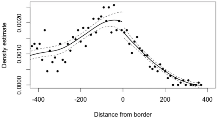
mial estimates of thegrowth in light intensity– the variable relevant for our difference-in-difference combined with RDD identification strategy described below – around the distance to the threshold before and after breakup are displayed. Figure 4 assesses the validity of the identifying assumption with the McCrory (2008) test for breaks in the density of the forcing variable at the treatment border with negative distances to state border for old states and positive distances for new states. The figure clearly shows that the density does not change discontinuously across the border, suggesting that for the window around the coverage border there seems to be no manipulation. This is to be expected given the firm exogeneity of the borders, but it is reassuring all the same.
We define a variable,Di, as constituencyi’s distance to the geographic borderd that splits each of these geographic location between old and new states. We then define an indicator for each AC for belonging to the new state as
Ti=1[Di≥d]. (3)
The discontinuity in the treatment status implies that local average treatment effects (LATE) are non-parametrically identified (Hahn et al. 2001). Effectively we compare outcomes for constituencies on either side of the geographic border that determined treatment assignment or being in a New State. Formally, the average causal effect of the treatment at the discontinuity point is then given by (Imbens and Lemieux 2008):
τa= lim
g→d+E[Yi t |Di=g]−glim→d−E[Yi t |Di=g] =E[Yi t(1)−Yi t(0)|Di=d], (4)
whereYi t is the satellite light density of constituencyi in yeart.
An important feature to note in the above-mentioned design is that the discontinuity is geographi-cal, i.e., it separates individuals (ACs) in different locations based on a threshold along a given distance-based border. Using (4) to estimate the causal effect would ignore the two-dimensional spatial aspect of the discontinuity. This is because theborder linecan be viewed as a collection of many points over the entire distance spanned by the border. For example, an individual located north-west of the bor-der is not directly comparable to an individual located south-east of the borbor-der. For the comparison to be accurate, each “treatment” individual must be matched with “control” individuals who are in close proximity to their own locationandto the border line. We address this issue as follows. We di-vide the border for each state into a collection of points defined by latitude and longitude spaced at equal intervals of 15 kilometers. We then measure the distance of each AC to the border and include polynomials of distance and its interactions with the treatment variable. We then condition on the post-breakup interacted, border segment fixed effects in all the specifications, so that only ACs within close proximity of each other are compared.36
The local average treatment effect can be estimated using local linear regression by including poly-nomials of distance to the border (controlling for border segment fixed effects) to a sample of units contained within a bandwidth distancehon either side of the discontinuity.
We additionally exploit the time dimension of our data as a further source of identification. The identification strategy described so far exploits differences across nearby bordering units, post state breakup to investigate the effect of breakup. Even then, it is possible that there is an underlying admin-istrative discontinuity at the border cutoff in the absence of breakup, since the geographical border was laid around existing districts. To address this issue, we use the observedjumpin outcomes to dif-ference out suchfixed, initial differences between units on either side of the border. Our identifying assumption is, therefore, that the jumps at the cutoff are not changing over time in the absence of
36See Black (1999), who first discussed the use of the border segments in a regression discontinuity framework. For a
Figure 3: Growth in light intensity after secession
The figure plots the local polynomial estimates of the growth in light intensity, defined as the difference in average light intensity post (2001-2009) and pre (1992-2000) the secession, around the threshold distance.
Figure 4: RD validity: density smoothness test for distance to state border
[image:20.595.104.471.494.696.2]treatment, so that the differenced local Wald estimators will be unbiased for the local average treat-ment effect.
Our overall identification strategy effectively combines the RDD design with a difference-in-difference approach. A key identifying assumption of this empirical strategy is that of conditional common trends before the secession for areas close to the border. We discuss this assumption further and ex-amine its empirical validity in Section 5.4.
With this in mind, the specification we estimate is
Yi t =αi+βt+γTi×Postt+δ 0
Vi t +ςs×Postt+"i t, (5)
whereYi t is the satellite light density of ACiin yeart. αiis the fixed effect for each AC. The variable of interest, the new state effect, is denoted by the interaction ofTi, being located in the new state, and Postt =1[t≥2001]. We control for border segment fixed effects,ςs (interacted withPostt to account for the panel dimension). The termsαiandβtrepresent constituency and time fixed effects respectively. TheVi t’s are defined as
Vi t =
1[Di<d]×Postt×(Di−d)
1[Di≥d]×Postt×(Di−d)
. (6)
The regressorsVi t are introduced to avoid asymptotic bias in the estimates (Hahn et al. 2001, Imbens and Lemieux 2008). Standard tests remain asymptotically valid when these regressors are added.
A panel fixed-effects estimator around the distance thresholds,h, is equivalent to using a uniform kernel for local linear regression, as suggested by Hahn et al. (2001). We consider several bandwidths, based on the optimal bandwidth calculations of Imbens and Kalyanaraman (2011), and for each we derive OLS-FE estimates using observations lying within the respective distance thresholds.
5 ESTIMATIONRESULTS
5.1 BORDEREXOGENEITY ANDBALANCINGTESTS OFCOVARIATES
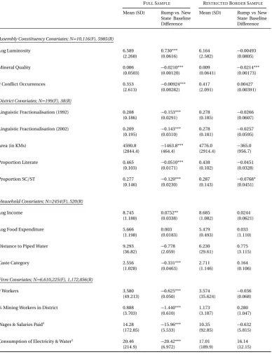
Our spatial discontinuity design compares ACs across borders, with the basic notion that differences in patterns of local activity, controlling for time-invariant characteristics before breakup can only be attributed to the secession rather than differences due to other factors. This in turn depends on the variation in observable attributes including human and physical geography. The demarcation of the borders here are historically determined, based on ethno-linguistic differences as they were present in 1947 at independence, or even earlier. If the historical demarcation implies a different settlement by these groups today, this in turn might pose a threat to identification.
that remains significant even within our restricted border-sample is the constituencies’ mineral en-dowments. However, we should expect a-priori such a difference and is the basis of our empirical ex-ploration that links secession to natural resources distribution. However to account for this difference, we use constituency fixed effects in our empirical strategy to difference out this time-invariant en-dowment. Additionally, we check the robustness of our results to differential mineral-specific trends (for e.g., price effects) and show that our results are not affected by this (in Section 5.3). In sum, our difference-in-difference strategy does control for fixed pre-breakup differences such as mineral en-dowment – this is less of a threat to identification than time varying differences reported below.
We also focus on district-level characteristics, and use information from the 2001 socio-economic census to examine two key characteristics, education and caste composition, that could influence outcomes. The table shows that for both variables, proportion of literates and proportion of back-ward caste population, the restricted sample differences between the rump and new state are small, and much lower compared to the full sample. We do find a small statistical difference in the percent-age of backward caste population in the restricted sample but show later (in Section 5.3) that the trend differential is not statistically significant, as required by the common trends assumption of our iden-tification strategy. We also find no significant difference in the average size of districts across borders, within the restricted sample. Another possible source of bias is the extent of fractionalisation based on linguistic differences across borders. Since the breakup was partly motivated by linguistic differ-ences, it is possible that the areas in the new states were linguistically more fragmented which could indirectly impact economic outcomes (Alesina et al. 2003). Using information from two rounds of the Language Atlas of India, we construct measures of linguistic fractionalisation based on Alesina et al. (2003), and find that the measure is stable and statistically not different between the rump and new-state bordering districts.
Next, we use information from the IHDS on income, consumption expenditures, measures of health (proxied by infant mortality) and public goods access (proxied by the distance to piped water), to see if these variables were different across border areas before breakup (year 1992 of the IHDS sur-vey). We conclude that they are not, in the restricted border sample. Finally, we examine firm-specific covariate differentials, combining data on all establishments from the Economic Census (year 1998) and supplementing it with information on a sample of firms from the Annual Survey of Industries (year 2001). Significant differences in employment or wage patterns could represent a threat to our identification as they could shift the distribution of economic outcomes post-secession. However, as Table 2 shows, we find that while significant differences exist in the full-sample, the restricted border sample means match well across all covariates, leaving small and statistically insignificant difference across borders.
5.2 RDD ESTIMATES
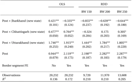
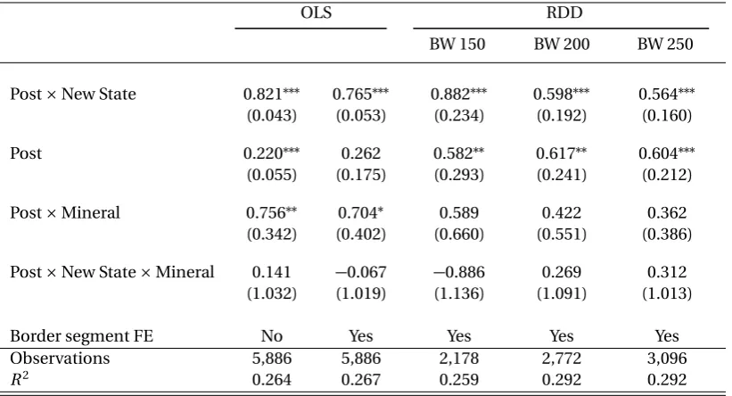
We begin with the overall effect of state breakup on the difference in luminosity in Table 3, before mov-ing on to our main results on how they vary with state-level natural resource abundance. The variable
Postcaptures the trend across states post breakup while ‘Post×New State’ captures the difference be-tween the new and rump states on average, post breakup. The first two columns of the table report the OLS estimate of breakup for the entire sample of ACs across all six states, reporting effects with-out and with border segment fixed effects. The naive OLS specifications suggest that while all states experience trend increase in luminosity, on average new states did better than the rump states.