Money market volatility, A simulation study

(1)

Michal Kempa

Money market volatility –

A simulation study

Bank of Finland Research

Discussion Papers

(2)

Suomen Pankki Bank of Finland P.O.Box 160 FI-00101 HELSINKI Finland + 358 10 8311 http://www.bof.fi

(3)

Discussion Papers

13

•

2006

Michal Kempa*

Money market volatility –

A simulation study

The views expressed are those of the author and do not necessarily reflect the views of the Bank of Finland.

* RUESG, Arkadiankatu 7 (PL 17), FIN-00014 University of Helsinki, Finland. Tel. +358-9-1912 8745, e-mail:

[email protected] and Research Department, Bank of Finland.

I would like to thank Hugo Rodrígues Mendizábal for Gauss code, Tuomas Välimäki, Alain Durré and participants of the seminars in the Bank of Finland and FDPE for comments and OP Bank Group Foundation for financial support.

(4)

http://www.bof.fi ISBN 952-462-284-X ISSN 0785-3572 (print) ISBN 952-462-285-8 ISSN 1456-6184 (online) Multiprint Oy Helsinki 2006

(5)

Money market volatility – A simulation study

Discussion Papers 13/2006

Michal Kempa

Monetary Policy and Research Department

Abstract

This paper analyses different operational central bank policies and their impact on the behaviour of the money market interest rate. The model combines profit maximising behaviour by commercial banks with the central bank supplying the liquidity that keeps the market rate on target.

It seems that frequent liquidity supplying operations represent an efficient tool to control money market rates. An averaging provision reduces the use of standing facilities and interest rates volatility in all days except for the last day of the maintenance period. Whenever banks have different maintenance horizons both the spikes in volatility and use of standing facilities disappear. The paper also compares two different liquidity supply policies and finds that the level of liquidity necessary to keep the rates on target depends on not only the aggregate but also assets values of individual banks.

Key words: Interbank market, interest rate volatility, central bank procedures, open market operations

(6)

4

Simulointitutkimus rahamarkkinoiden

korkovaihteluiden määräytymisestä

Suomen Pankin tutkimus

Keskustelualoitteita 13/2006

Michal Kempa

Rahapolitiikka- ja tutkimusosasto

Tiivistelmä

Tässä tutkimuksessa tarkastellaan keskuspankin likviditeetinhallintajärjestelmän vaikutuksia rahamarkkinoiden korkoihin. Tarkastelujen teoreettinen malli kuvaa voittojaan maksimoivia pankkeja sekä keskuspankkia, joka likviditeetin tarjonnal-laan pyrkii pitämään rahamarkkinoiden korot tavoitetasolla. Tutkimuksen tulokset osoittavat, että rahamarkkinakorkojen vaihteluita voidaan hallita useasti toistuvien rahamarkkinoiden likviditeettioperaatioiden avulla tehokkaasti. Varantojenpito-jakson viimeistä päivää lukuun ottamatta vähimmäisvarantojen keskiarvoistami-nen vaimentaa korkovaihteluita ja vähentää keskuspankin maksuvalmius-järjestelmän käyttöä pankeissa. Toisistaan poikkeavien varantojenpitojaksojen tapauksessa huipentumat sekä korkovaihteluissa että keskuspankin maksuvalmius-järjestelmän käytössä häviävät. Työssä verrataan myös kahta vaihtoehtoista likviditeetintarjontamallia ja päätellään näiden tarkastelujen perusteella, että voidakseen vakauttaa korot tavoitetasolle keskuspankin on markkinoiden likviditeettitilanteen lisäksi otettava huomioon yksittäisten pankkien maksu-valmius.

Avainsanat: pankkien väliset rahamarkkinat, korkovaihtelut, keskuspankin menettelytavat, avomarkkinaoperaatiot

(7)

1 Introduction

The view that the central bank (CB) exerts an influence over the economy by using interest rates as a direct tool has now been widely accepted for some time. The exact mechanism of control over the interest rate, or so called the operational policy has however attracted much less attention and very often is taken for granted. This particular research niche has recently seen some revived interest resulting in a series of publications; many questions however remain still open.

The operational policy targets the level and volatility of the interbank market interest rates, and basic instruments at the CB disposal include: an obligatory reserve requirement, open market operations (OMO) and lending/deposit facility. So far no golden rule for the eﬀective operational policy mix has been found. Indeed, countries over the world have decided in favour of very diﬀerent setups and none of them can claim perfect control, even though all are successful in setting the rates on target level in the long term. There are several issues to consider, such as the balance between intensity (or willingness) of the central bank intervention and the volatility of interest rates. Still countries using similar tools experience systematic patterns of interest rate behaviour, overcoming country specific features. For example, a system with an averaging reserve requirement, infrequent (ie not daily) open market operations and a wide channel of standing facilities (similar to the one present in Eurozone and the US) apparently experiences fairly low volatility during the maintenance period, but risks regular spikes around the end of the periods (see Figure 1 that presents the time series of target and market rates). On the other hand, countries such as Canada or Sweden, supplying the liquidity through daily OMO and narrow standing facilities rates (thus running a more active policy) enjoy much less volatility of interest rates at the cost of a less active interbank market and a higher degree of central bank intervention (see Figure 1). Somewhere in the middle is the UK with its system of an one-day maintenance period and daily interventions.

The similarities in patterns of interest rate behaviour between markets as different as the US and the European, justify several research questions. What is the impact of different aspects of operational policies on the behaviour of the money market? How does the volatility of interest rates change when a different mix of the operational policy instruments is applied? What is the impact on the use of central bank standing facilities be used? Suppose the central bank commits to a specific policy — what is the volume of open market operations that would keep the rates on target? The usual approach is to target the aggregate liquidity, without consideration of the individual shock distribution across banks. What if the information about the distribution was actually included in the decision process? The following paper addresses those questions.

The money market despite its central position in the central bank policy, has only recently started to attract appropriate amount of attention. An excellent and extensive introduction to thefield is presented by Bindseil (2004). Hamilton (1996) expressed formally one of the most important hypothesis related to the market: money market funds should be perfect substitutes

(10)

(11)

in all days of the reserve requirement period, which implies the interest rates should satisfy martingale property. He then analysed the data series for the US and found it did not hold, which sparkled lots of research on that topic. Most of them was based a single bank’s profit maximising behaviour in a general equilibrium setup, in a spirit of Poole (1968). For the Eurosystem an interbank model was designed in Pérez-Quirós and Rodríguez-Mendizábal (2001), Gaspar et al (2004). Analogous references for the USA are Bartolini et al (2001, 2002), both analyses, however, strictly tailored to country-specific features. They have concentrated on the volatility of the interbank interest rates in diﬀerent stages of the maintenance period as a phenomenon crucially dependent on the obligatory reserve requirement. In these models the emphasis is on the commercial bank’s behaviour, while the role of the central bank as the initial supplier of the liquidity is very often simplified by assuming the starting assets as given.

Models that overcome these limitations were created by Välimäki (2003), Moschitz (2004) where the supply of the funds by central bank is included as well. Those papers do not however explore the details of the optimal level of liquidity. The model which is closest to mine paper is Bartolini and Prati (2003) where they investigate market volatility under a spectrum of different policies for liquidity supply, using similar methods. In their model OMO take place every day, with its volume chosen so to minimise the deviation from the target rate. Without any restrictions that approach leads to the full control over the rates which is not realistic. That result is replicated as one of the sub-cases in this study as well. To bring their study a bit closer to reality then, they constrain the central banks actions by introducing some arbitrary limits on the volume of the interventions. In this paper a different approach is used where the central bank is restricted by the operational policy details (such as timing or frequency of OMO) rather than its ability to offset liquidity shocks. Bartolini and Prati (2003) do not also analyse the impact of periodic OMO or effects of the policy setting neutral liquidity.

Finally the regime where the banks have diﬀerent maintenance period dates has been discussed only in Cox and Leach (1964) but without rigorous analysis. The paper contributes to the existing research in several ways. First, it simulates the behaviour of money market under diﬀerent regimes within one framework. This provides an opportunity for a clear comparison of policy performance measured in terms of the use of the standing facilities or volatility of interest rates.

Second, active central bank liquidity supply policy, provides a benchmark against which neutral market liquidity targeting can be compared.

Third, the regime with overlapping maintenance periods has not been properly examined before in the literature, while it is a potentially very interesting case combining some of the benefits and costs of existing policies.

This study is structured in the following way. Section 2 contains the basic model structure. Sections 3 and 4 include details on the liquidity demand (commercial banks) and supply (central bank) side of the market. In section 5 I present the results for diﬀerent simulations andfinally section 6 concludes.

(12)

2 Model overview

Every day banks are involved in scores of transactions, resulting in changes of their own as well as market liquidity. From the perspective of individual banks some can be predicted in advance with a fairly good accuracy — an example would be maturing securities — but others constitute a stochastic shock. The money market in this world is used to help to manage liquidity and moderate the liquidity shocks. The banking market is governed by standard economic rules, where excess liquidity depresses the interest rate and free funds shortage drives it up. A policy targeting the level of the interest rates can therefore be implemented through channels that control the market liquidity.

The market liquidity is settled during open market operations before the interbank trade is closed, which is incorporated in the structure of the model by using simple two-stage framework. In the early stage the central bank sets the value of market liquidity, and in the latter one banks trade excess resources at the market rate. More specifically the timing of events in the market is as follows:

1. A commercial bank starts the day with a balance at the CB account mt.

2. Open market operations start, as a result, the bank’s current account balance changes byθt.

3. An early stochastic shockε1t occurs

4. The interbank money market opens with banks trading assets bt at an

market clearing interest rate it.

5. A late stochastic shock ε2t occurs after no trade is possible anymore.

After that, the final bank balance in the central bank is calculated, and constitutes the opening balance for another day. Depending on the sign, the bank automatically refers to either the deposit or the lending facility.

mt,1 θt ε1t bt ε2t mt+1,1

−−−−−−−−−−−−−−−−−−−−−−−−−−−−−−−→

Combining the steps 1—5 results in the following diﬀerence equation

mt=mt−1+bt+θt+εt (2.1)

where mt denotes the assets in the central bank, bt denotes net change in

interbank lending,θtis the balance of open market operations andεt=ε1t+ε2t

is the sum of stochastic shocks during a day.

The shocks capture the imperfect information that is faced by both central bank and commercial banks and here are assumed to have the same variance

σ. One of the shocks,ε1t , apart from shifting the liquidity between banks has

also an aggregate impact on the market. In the a real life this occurs whenever there is a change in balance of so called autonomous liquidity factors1 _{such as} 1_{Bindseil (2004) provides a following de}_fi_{nition of autonomous liquidity factors: ‘All items}

in the balance sheet of the central bank that do not reflect monetary policy operations, or the reserve holdings (that is, the ‘deposits’ or ‘current accounts’) of banks with the central bank’.

(13)

currency balances or government accounts. The other shock,ε2tis idiosyncratic

and reflects the balance of transactions performed between banks during the day.2 They satisfy Pn_i₌₁ε1ti 6= 0 and

Pn

i=1ε2ti = 0.

The interbank trade is driven by profit maximising banks that cash the profits on lending, but are subject to two constraints:

1. The end of the day balance at the central bank account must stay non-negative — otherwise, the bank is forced to automatically use the Central Bank lending facility

2. An average level of reserve requirement must be satisfied throughout the maintenance period.

More detailed explanation is included in the following section, but it might be useful to look into one-period commercial bank expected profit function

Πt=itbt−Et(ct) (2.2)

where it denotes the interbank interest rate, bt bank choice of lending value

and Et(ct) is the expected cost of using the standing facilities after the final

liquidity shock arrives. The profit maximisation problem has to be solved in an environment with stochastic liquidity shocks (denoted εt before). Note

that from the bank perspective the early shock is less interesting since it can be oﬀset during the interbank trade. Any mistakes in calculations of the late shock however force the bank to use costly standing facilities.

The central bank goal is to keep the market interest rates as close to the target as possible. To achieve it, it supplies the liquidity both actively, using open market operations (denoted θ), and passively, using standing facilities. Depending on monetary policy setups, the extent and frequency of open market operations may diﬀer, but their value is set so as to keep the market rates on the target. The deposit and lending facilities help the banks to manage the uncertainty. Should an individual bank’s current account balance turn negative in the end of the day, the bank recourses to (marginal) lending facility. If the account value exceeds the amount of reserve requirement, the bank settles a deposit. The interest rates for standing facilities are accordinglyil _{for lending}

and id _{for deposit and they are tied to the target by the assumption that the}

target rate i_∗= (il+id)/2 ie lies exactly in the middle of the channel system (as is the case for example for ECB).

In practice averaging provision reserve requirement means that the bank has to accumulate a fixed amount of funds on its account during the maintenance period. Denote this amount byRanddtby the time tdeficiency,

dt satisfies

d1 =R (2.3)

2_{In the Eurozone, the late liquidity shock results usually from smaller transactions hence}

its relative lower significance comparing to the early shock. In the simulation however, for the computational reasons these two have been assumed identically and independently distributed.

(14)

di = ⎧ ⎨ ⎩ di−1 if mi <0 di−1−mi if 0< mi < di−1 0 if mi > di−1 (2.4)

for anyT _≥i_≥2, whereT is the end of the maintenance period. IfdT > mT+

εT the bank does not satisfy its reserve requirement at the end of the day T,

and it has to refer to the central bank standing facilities without extra penalty. There is no interest capitalisation and time span is only one maintenance period. No change in the regime or level of target interest rate is assumed in the paper.

3 Demand side

This section presents the model of the commercial banks behaviour in the interbank market. The chapter follows quite closely the works of Välimäki (2003), Pérez-Quirós and Rodríguez-Mendizábal (2001).

3.1

No reserve requirement

Without reserve requirement, there is no significant diﬀerence between diﬀerent days. The situation is similar on the last day of the maintenance period in the regime with reserve requirement. The expected profit function of the banks takes the one-period form

Vt= max bt

Et(Πt) =Et(itbt−ct) (3.1)

where itbt stands for the profit from interbank lending and E(ct) denotes

expected cost given by

E(ct) =il ∙Z −mt+bt−θt−ε1t −∞ (mt−bt+θt+εt)f(ε2t)dε2t ¸ − id ∙Z ∞ −mt+bt−θt−ε1t (mt−bt+θt+εt)f(ε2t)dε2t ¸ (3.2)

where f(ε2t) denotes the density function of the shock. The expected cost

for individual bank is calculated using the fact that whenever the negative liquidity shock does not exceed the bank’s current account balance at the end of the day (given by mt+θt−bt−ε2t), the remaining assets are remunerated

at id _{interest rate. Otherwise bank is forced to use borrowing facility at the}

rate il_.

Using the Leibniz Rule and first order conditions one arrives at the well known result (Proof in the appendix A)

it=id+ (il−id)Fε2t(bt−mt−θt−ε1t) (3.3)

(15)

with Fε2t(.) as the associated distribution function of the ε2t late shock. The interbank interest rate is equal to the expected cost of using the CB lending/borrowing facility. (3.3) holds for all the banks and the inverse of normal distribution functionF_ε−₂1_t exists, so one can aggregate the equation to obtain following result

it=id+ (il−id)F(−Mt−Θt−ε1¯t) (3.4)

Bank loans net up to zero,Mt=

Pn

i=1m

i

t is the aggregate amount of funds at

the account in the central bank in the beginning of a day and ε1¯t =

Pn

i=1ε

i

1t

is the aggregate shock value. This result indicates how the central bank, by controlling the aggregates, can influence the level of interest rates, without worrying of the distribution of assets across banks. This is a very strong result, giving support to the policies of several central banks that tend to use only aggregated liquidity information when calculating the allotment.3

Note, however, that it holds only under fairly strong assumptions (identical distribution, no reserve requirement) that do not necessarily survive extensions into more general settings.

Before moving further, one last remark. The case described in this section has a straightforward extension to a regime with reserve requirement but

without averaging provision (as hitherto in the United Kingdom). It is enough to add a constant term, equal to the required reserves, to the expression in brackets in (3.4) in the last day of maintenance period and leave the equations in other days unchanged.

3.2

Reserve requirement

3.2.1 Last day of maintenance period T

In the last day the situation is very similar to the case above, except for the reserve deficiency as an additional termdT in the cost equation

E(cT) =il ∙Z ₋mT+bT+dT−θT−ε1t −∞ (mT −bT +dT +θT +εT)f(ε2T)dε2T ¸ + −id ∙Z ∞ −mT+bT+dT−θT−ε1t (mT −bT +dT +θT +εT)f(ε2T)dε2T ¸ (3.5)

Solving the first order conditions associated with the optimisation problem (3.1), explicitly gives the value of optimal borrowing at rateiT

iT =id+ (il−id)F(bT +dT −mT −θT −ε1T) (3.6)

This expression is essentially the same as eq. (3.3) with the termdT being only

diﬀerence. Note that since dT ≥ 0, the amount the bank is willing to lend at

some interest rate level i, with the same asset m and OMO θ volume, will be

3_{In case of the ECB, so called benchmark allotment value is calculated by adding up}

the realised and expectedfigures for aggregate deficiency and autonomous liquidity factors (past and predicted) from one OMO to another.

(16)

lower in the regime with reserve requirement than without. This result is quite intuitive, but it has a direct implication. Once the equation is aggregated — similar to previous section — one gets

iT =id+ (il−id)F(DT −MT −ΘT −ε1¯T) (3.7)

with the aggregate borrowing cancelled out. Now the interest rate is a function of large aggregates. Hence the following property holds. In the last day of the maintenance period, the distribution of the individual shock among banks has no impact on the interest level and neutral market liquidity results in the rates in the middle of channel system. The neutral liquidity is defined as the level of funds that will be just enough to satisfy reserve requirement. The last part of the property results from the normal distribution assumption (F(0) = 1/2) and often is used as a basis for the central bank liquidity supply policy. This issue is discussed in more detail later on.

3.2.2 Days before end of maintenance period t<T

Let’s move now to the earlier stages. The value function in Bellman’s equation takes the form

Vt= max bt

Et(Πt+Vt+1) = max

bt

Et(itbt−ct+Vt+1)

The interest rate that solves that problem for each individual bank can be shown (check Pérez-Quirós and Rodrígues-Mendizábal (2001) for proofs) to satisfy it=ilF(bt−mt−θt−ε1t) | {z } 1. +id[1₋F(bt+dt−mt−θt−ε1t)] | {z } 2. − Z bt+dt−mt−θt−ε1t bt−mt−θt−ε1t ∂Vt+1 ∂dt+1 f(ε)dε | {z } 3. (3.8) and ∂Vt ∂dt =₋id[1₋F(dt−mt−θt−ε1t)] + Z dt−mt−θt−ε1t −∞ ∂Vt+1 ∂dt+1 f(ε)dε (3.9)

The intuition behind these results is as follows: marginal benefits (it)are equal

to the weighted cost of: 1. referring to the lending facility (when the shock exhaust all the funds at the current account), 2. deposit facility (the shock is high enough to exceed the required reserves) and 3. the impact of decreased deficiency today on the profits in the future (the shock value keeps the balance positive, but does not exceed the deficiency).

Contrary to the case without reserve requirement, the optimal borrowing value cannot be calculated explicitly from (3.8). That means the market clearing condition must be derived using numerical methods.

Recall the aggregation procedure used to calculate equation (3.4) for the last day of maintenance period. The single market rate implies the liquidity

(17)

value(bT +dT −mT −θT −ε1T) for all banks was the same, so the interbank

market (termbt) only function was to equalise the liquidity among banks. That

also allowed for easy aggregation and, with the assumption of shock normal distribution, observation that neutral liquidity leads to the markets rate in the middle of channel system. An inspection of equation (3.8) reveals that it is not the case anymore in the periods preceding the end of maintenance period. The banks will consider not only current liquidity position, but also future implications. That reflects the phenomena pointed out by Pérez-Quirós and Rodríguez-Mendizábal (2001) ie banks care about the future probabilities of referring to standing facilities, more specifically the increased probability of being forced to use deposit facility once the reserve requirement buﬀer is lost. In some extreme cases (a bank hit by a series of shocks) the last term might be much more important than current liquidity which might have profound consequences for the value market liquidity that would set the rates on target. These issues must be taken into consideration when designing the optimal policy setup.

3.2.3 Diﬀerent settlement dates

Finally, I also want to look into the case where banks are required to maintain the reserve requirement during a maintenance period, but the end of the period is diﬀerent for the groups of banks. That would allow the banking sector to operate as a whole with a lower total amount of funds and cancel the regular spikes presently observed at the end of the maintenance period. In principle, bank policy still follows the same equations (3.6) and (3.8), but the diﬀerence shows up on the aggregate level now. The periodic spikes in this setup will be smoothed. No predictions however can be made about the magnitude of volatility.

A potential weakness of this type of regime has been raised by some policy practitioners: it seems that the banking sector would have the possibility to transfer the liquidity to the banks that end the maintenance period, and ignore the reserve requirement in every other day. At first sight it seems that such a behaviour would vastly reduce the structural deficit of funds which is supposed to be the basis of eﬀective operational policy. Taking a closer look at averaging provision however helps to realise that these concerns are misplaced. Aggregate current account holdings hardly ever exceed the daily portion of the reserve requirement (in the model — exactly match) of the whole banking sector, and hence there is no surplus liquidity on the market.

Another problem may arise whenever there is a change in the target rate. Taking the ECB as an example, the changes of rates have been recently synchronised with the maintenance period, in order to prevent speculative accumulation of liquidity during the period. Letting the end of the maintenance period dates to diﬀer will obviously increase the level of such a wasteful activity.

(18)

4 Supply side

The supply side — the amount of liquidity the central bank injects into the market — will be modelled following the approach introduced by Välimäki (2003) and later on by Moschitz (2004).

First of all, the CB facing a choice how to supply the excess liquidity has to consider the following trade oﬀs :

1. Daily OMO allow for great flexibility and swift adjustments but might pose some operational and technical problems,

2. Late liquidity supplying operations (fine tuning or narrow channel system) essentially set the end of the day rate at specified target, but take away some incentives for trading on the interbank market (since the penalty for using CB facilities is much lower)

3. The reserve requirement allows bank for more flexibility when faced by the shock, since it works as a buﬀer. Should the bank run short (or excess) of funds at the end of the day, instead of referring to CB standing facilities it can ignore it and make up for it later during maintenance period. The problems however occur around the end of the maintenance period, when the volatility and level of rates becomes much higher.

An interesting alternative — mentioned already above — that has not however been implemented in practice, would be to change the averaging provision regime and allow for diﬀerent settlement dates between banks.

These trade-offs set the frames for the present analysis. By comparingfinal interest rates and values of CB intervention in different regimes it is possible to evaluate the efficiency of each policy mechanism.

In terms of the model, regardless of the applied policy, I assume the central bank goal to minimise the deviation from the fixed target rate i∗_. _More specifically, the CB is assumed to operate with a quadratic objective function

min E " _T X t=1 (it−i∗)2 #

The target rate is linked to the commercial banks behaviour by setting the middle point of the channel system. Also banks are assumed to expect the future rates equal to target rate. This assumption is justified by ignoring the possibility of changes in the target rates in this paper.

(19)

To achieve its target the central must find

1. the amount of liquidity that would induce the interest rate to remain as close as possible to the target...

2. while using the information about the expected changes in the autonomous liquidity factors and remaining deficiency.

In this study I do not analyse potential additional central banker’s motives such as supervision of the banking sector or its credit risks, hence the Central Bank facilities (including OMO) will always be available no matter what is the value of assets of an individual bank.

Depending on the frequency of OMO the model time horizon T will take diﬀerent values. In case of daily OMO the CB will be one period looking, while in case of single OMO T will cover whole maintenance period. Even though the model assumes the CB carries no cost of OMO, there are still some other restrictions that render the problem non-trivial. The most important is that the CB can not simply assign a individual allotment value but rather an aggregate. In other words, the central bank cannot decide on how much liquidity each bank receives separately and it must count on the market to distribute it eﬃciently. There is also another time lag (and shock realisation

ε1t) before CB allotment decision and the interbank market close, so if the

individual liquidity distribution matters, there will be some deviation from the target.

The exact allotment policy in this model is simplified to divide the aggregate amount equally to each banking player. Since the money market opens after the allotment, banks are free to trade any excess liquidity among themselves. Hence this assumption is not particularly restrictive.4

4.1

No reserve requirement

Whenever OMO are performed on a daily basis, the aggregate value of the shock can be corrected by the CB on a daily basis. Available assets for each bankmt+θt are set by the central bank and the problem of finding the right

allotment value reduces to solve (3.4), repeated below

it=id+ (il−id)F(−Mt−Θt)

The symmetric corridor with the target rate in the middle, and normal distribution implies the solution hinted already in section 3.1

F(₋Mt−Θt) =

1

2 (4.1)

or using normal distribution property

−Mt−Θt= 0 (4.2)

4_{Actual tender bidding policies of individual banks have been analysed by Välimäki}

(20)

so the CB should attempt to sweep away any excess liquidity.

The situation is diﬀerent if the OMO take place once a while, say everyTth

period. The target then would be to set theaverage rate during that period ie

i∗ =E0

PT

t=0it T

With such a policy, just offsetting predicted liquidity shock might encounter a major problem. Suppose the CB predicts the aggregate value of autonomous liquidity factors duringT periods to reach some value (say, negative), and sets the amount of funds allotted in the beginning so as to offset the sum of the shock. Clearly, in thefirst period that would mean that the market is flooded with money and drive the rates all the way to the deposit facility rate. Only in the last period, the shock will befinally balanced (if the predictions proved true) and the rate will reach the target. Indeed, the simulation results indicate that the optimal allotment value differs from such a policy.

4.2

Reserve requirement

Regardless of the frequency of CB intervention (OMO), the question of the optimal level of liquidity arises also with the reserve requirement present. On one hand, more liquidity is needed on the market (higher early CB intervention), on the other, the liquidity can be used as a cushion against volatile shocks (less late intervention).

Unfortunately this model oﬀers an analytical solution only for the problem in the last day of the maintenance period that is a simple modification of (3.7). In all other cases, the CB will face a simple optimisation problem, to be solved for the optimal amount of liquidity allotment. The details are included in the section describing a simulation study.

Before the simulation study results, let us come back to the problem of targeting individual vs aggregate liquidity. The problem is not a trivial issue, since most popular operating procedures concentrate usually on the aggregate market shortage or excess. From the results presented so far it seems however that ignoring the information about individual liquidity can only work properly in a few regime types (eg without reserve requirement) but otherwise it does matter. This issue has been also discussed by Bindseil (2004) in relation to the excess reserves tracking.

First of all, in the last day of maintenance period, the individual assets history is indirectly included in the aggregate deficiency DT, calculated from

the individual deficiencies from earlier dates and might differ even though the market asset value at time T and T ₋1 and the aggregate shock realisation is the same. A simple example with two banks and two periods illustrate the argument. Two cases with same aggregate values of assets or shocks, but different distributions of starting deficiency result in very much different outcome on the market.

(21)

Day T-1 Day T assets deficiency shock assets deficiency

bank A 5 1 10 15 0

bank B 5 19 -10 -5 19

Total 10 20 0 10 19

Case1.

Day T-1 Day T

assets deficiency shock assets deficiency

bank A 5 10 10 15 0

bank B 5 10 -10 -5 10

Total 10 20 0 10 10

Case 2.

In the example the aggregate value of assets (10 units) is just enough to satisfy the reserve requirement (total deficiency of 20 spread into two days) hence the central bank not concerned about individual assets would simply refrain from any intervention (the liquidity shock netting oﬀto 0). Sticking to that policy works well in case 2., since the market ends the maintenance period exactly with neutral liquidity. That, according to (3.7) results in rates on target. Similar policy fails however to provide the market with enough liquidity in case 1. That, according to the same formula will result in the market rate higher from target.

A real-life situation reflected in the example above could appear in the regime with periodic OMO, when there is no possibility to alter market liquidity in the last day of maintenance period. However a regime that would allow for additional liquidity inflow in the last day of maintenance period, (in a form offine tuning or additional open market operations) would still be capable of making necessary correction. This leads to an important observation of the paper: not only the frequency but also the timing of the operations matter. This view is apparently shared by the ECB, where the late liquidity operations have been recently launched.

To conclude this section, the most important finding is that not only aggregate value, but also the distribution of the shock among the market participants might be important. Simple example illustrates the case where the same initial aggregate market liquidity and deficiency might result in very diﬀerent market clearing rates. This can be managed by appropriate timing, such as introduction of some form of late interventions.

5 Simulation study

In order to show the aggregate banking sector behaviour, with each bank borrowing given by 3.8 I turn to numerical methods. In this section the design and results of the simulation study are presented.

The purpose of the paper is to analyse the impact of diﬀerent market design on the behaviour for the interbank market. In practice it means I am going to keep the interbank money market (demand structure) unchanged, while

(22)

experimenting with various ways to supply the liquidity (supply structure). More precisely the profit maximising behaviour and the exogenous shocks are going to be kept fixed, while the value and timing of open market operations or reserve requirement regime will be altered.

The elements of the operational policy analysed are:

1. The averaging provision regime, with three possible cases

(a) Traditional regime with the same maintenance period for all banks, (b) Regime without any reserve requirement at all

(c) Regime with diﬀerent maintenance periods for groups of banks,

2. The frequency of the open market operations (early liquidity supplying operation)

(a) Daily supply (daily OMO)

(b) Periodic supply (once per maintenance period)

3. The volume of the open market operations

(a) Supplying an amount equal to the shortage of funds to the market (zero-excess liquidity)

(b) Supplying the value of funds using a simple optimisation algorithm (optimised liquidity).

The reasons these regimes were picked are bound to their resemblance to the actual policies of central banks. For example, the ECB uses the averaging provision reserve requirement, periodic liquidity supply with the value equal to the predicted forthcoming autonomous liquidity factors (aggregate shock in the model) and remaining deficiency.5 _{On the other hand, Sveriges Riksbank}

uses no reserve requirement with daily liquidity operations.

For clarity, the simulation has been divided into 3 sections corresponding to diﬀerent reserve requirement policy, and then each of 4 regimes is analysed:

• I. Daily OMO, zero-excess liquidity; • II. Periodic OMO, zero-excess liquidity; • III. Daily OMO, optimised liquidity; • IV. Periodic OMO, optimised liquidity

5_{ECB however performs four liquidity supply operations every maintenance period.}

(23)

For each analysed variant of the policy, the following parameters are of particular interest:

1. The volatility of the interest rate measured during the simulation runs. 2. The volume of trade on the interbank market, measuring how eﬃcient the

banking sector deals with smoothing out the eﬀects of liquidity shocks. Ideally each individual bank should trade the amount that would leave it with a neutral liquidity position.

3. The recursion to deposit and lending facilities of the central bank, showing the level of late intervention

4. The average liquidity left on the market after open market operation (measured as the sum of liquidity shock and liquidity allotment)

The results are reported in the following sections.

5.1

Method outline

In what follows an outline of method is presented. The details are included in the appendix.

Following the approach of other researchers in thisfield, commercial banks expectations of the interest rates will be given by the central bank rates. These beliefs are confirmed in the data, where indeed the hypothesis of significant diﬀerence between mean interest rates in any day of the maintenance period is rejected (see eg Moschitz (2004) for EMU data).

There are no frictions on the market that in the real life could are likely to occur for example due to cross-border cost of information. Hence, the markets always clear.

The simulation follows the model outline meaning it is divided into demand and supply part. The algorithm takes the following form (details can be found in the appendix):

Step 1. The central bank sets a level of aggregate liquidity (supply of funds).

Step 2. The market clearing rate is calculated (where the aggregate borrowing ends close to zero)6_.

Step 3. Should the market rate end up away from the target, the initial allotment decision is updated .

When the central bank calculates expected market rate in Step 2., it has some initial idea about distribution of liquidity, but it may change by the time the market opens. This reflects the fact that in reality central banks have developed very accurate techniques to predict the aggregate liquidity shocks, but do not try to guess individual value. This distinction is reflected in the simulation design as well, by allowing two shock realisations. One of them has an aggregate value diﬀerent from zero (like changes in autonomous liquidity

6_{I would like to thank Hugo Rodríguez Mendizábal for providing the code used in the}

(24)

factors), but known by the central bank. The second part of the shock is purely idiosyncratic7_{, and it is excluded from the central bank optimisation}

algorithm.

The presentation of the simulation results will be divided into groups, following the scheme introduced early in this paragraph. For the simulations the commercial bank assets value mt = 200 units is used, with the liquidity

shock variance (ε1t and ε2t) equal to 60. There are N = 10 banks on the

market, and the reserve maintenance period is 3 days. During that period each bank is obliged to accumulateR = 3_∗mt= 600 units of money, so there

is enough liquidity on the market. The choice of the parameters has been arbitrary and roughly follows the values used in the existing research.

5.2

Averaging reserve requirement

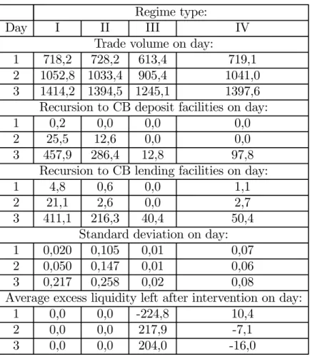
I start the presentation of the results from the case when the commercial banks must satisfy the reserve requirement with averaging provision. Within that framework, there are several interesting extensions, namely the impact of daily or periodic OMO and which algorithm for funds allotment works better. Note that one of the cases (no. II in Table 1), ie periodic, zero-excess liquidity OMO reflects quite closely the policy run by the ECB, hence its relative importance compared to the other cases.

The volume trade on the market diﬀers slightly between allotment regimes, but is not influenced by the frequency of OMO. This result is quite intuitive — the value of trade depends on the variance of assets among banks (all have to satisfy the reserve requirement of the same value) that are using the trade to compensate liquidity shocks. The OMO in this setup does not influence that variance (the target is the aggregate liquidity) hence its neutral impact on the trade volume.

The increase in volume can still be observed as the time passes. This is related to same issues brought up before: all banks in the model start the day with the same assets, but as the shock realisations build up, the variance of assets among the banking sector increases. In general, the volume of trade in that case will be used later on as a benchmark for measuring the eﬃciency of interbank market, with diﬀerent policy setups.

7_{This shock re}_fl_{ects the balance of payments of transactions taking place inside the}

banking sector.

(25)

Regime type:

Day I II III IV

Trade volume on day:

1 718,2 728,2 613,4 719,1 2 1052,8 1033,4 905,4 1041,0 3 1414,2 1394,5 1245,1 1397,6 Recursion to CB deposit facilities on day: 1 0,2 0,0 0,0 0,0 2 25,5 12,6 0,0 0,0 3 457,9 286,4 12,8 97,8

Recursion to CB lending facilities on day: 1 4,8 0,6 0,0 1,1 2 21,1 2,6 0,0 2,7 3 411,1 216,3 40,4 50,4

Standard deviation on day: 1 0,020 0,105 0,01 0,07 2 0,050 0,147 0,01 0,06 3 0,217 0,258 0,02 0,08

Average excess liquidity left after intervention on day: 1 0,0 0,0 -224,8 10,4

2 0,0 0,0 217,9 -7,1 3 0,0 0,0 204,0 -16,0

Table 1: Averaging provision reserve requirement

Let’s move on to the use of standing facilities. The use of both facilities — at least whenever the optimisation algorithm is used — seems limited, with the jump on the last day of maintenance period. This is plausible; early on it is still possible to use the funds to satisfy reserve requirement, so there no need to apply for a deposit. At the same time positive balances serve as a buﬀer from negative shocks, preventing the lending facility from being used. All these advantages vanish in end of the maintenance period and result in increased spike that is also observed in example in Eurozone data (the average recursion to lending facilities in the period 1999—2005 was roughly 5 times higher on the last day of maintenance period than in other periods; for borrowing facility that ratio was around 9). Note that whenever the optimisation algorithm is used for determine the allotment value, the recursion to standing facilities is much lower.

Next entry in the Table 1. refers to the volatility of the interest rates on different days of maintenance period. First of all there is a vast difference between daily and periodic OMO case. This is not surprising: the payoff between frequent intervention and rates volatility has been widely acknowledged in the literature.

The model predicts that the volatility is increasing toward the end of the period, especially in the last day. That again is in line with the data (in Eurozone, the variance of EONIA rate is on average 5 times larger comparing to other days) and all previous research. This result becomes even more intuitive once one looks back at plotted demand functions (figure 2). In the last day of

(26)

the maintenance period the prices elasticities are significantly larger compared to other periods, which means that the interest rates are going to respond much more to the same shock value comparing to earlier days. Intuitively, this result has to do with the fact that 1) At least some banks in the market have already satisfied the reserve requirement and hence lost the buﬀer 2) the others banks balance, to avoid using expensive lending facility must not only remain positive (as in previous days) but also exceed the deficiency value.

Note that the volatility of the rates differs significantly between different allotment regimes, which brings me to the lastfigures in the table ie the volume of liquidity required for the interest rates to stay on target. Remember that in thefirst two regimes analysed (namely I. and II.), the amount of liquidity was just enough to offset the liquidity shock, while in the other cases (III. and IV.) it was recalculated based on optimisation algorithm for each iteration separately. From the simulation run it seems that even such a simple algorithm performs better comparing to simple zero-excess liquidity policy. Particularly interesting are the values of intervention in case of daily OMO. It seems that different days of the period require different sign of intervention ie the early stage requires liquidity shortage, then neutral liquidity in middle stage to finally move to liquidity surplus in the late stage.

This result is related to the phenomena pointed out by Pérez-Quirós and Rodríguez-Mendizábal (2001) where they analyse the German money market before 1999 and notice that the rates tended to be higher in the late days of the maintenance period, hence the liquidity at the end of the period must be more valuable. Their explanation is that early in the maintenance period, in order to enjoy buﬀer of required funds banks deliberately maintain lower liquidity (suppressing the rates level), a trend that is reversed toward the end of the period.

There is also another explanation for that, referring to section 4.2. Suppose the market as a whole has enough liquidity to satisfy the reserve requirement. Suppose further that one commercial bank is hit by a series of positive liquidity shocks which results in that bank fulfilling its obligations for that maintenance period. Now, any positive balance it will happen to hold until the end of the period will be deposited in the Central Bank and will not contribute toward satisfying global (market) deficiency. That however means that the rest of the market will be faced with shortage of liquidity, driving the rates above target level. In other words, the use of deposit facility depletes the pool of funds that banks use to satisfy reserve requirement. Obviously the problem will be more severe toward the end of the period. An active CB policy (as the one using the optimisation algorithm) would incorporate that fact in calculating the optimal value of liquidity allotment which contributes to its overall better performance. This again, provides also additional support to the ECB policy of late interventions (called end-of-theperiodfine-tuning operations).

To summarise the findings of that section, the most important result is that the neutral liquidity provision policy, just oﬀsetting the liquidity shock can be improved by even relatively simple optimisation algorithm. Also daily OMO tend to prevent the rates from excess volatility and but require higher level of the central bank intervention. Daily OMO require also changing the market liquidity in diﬀerent stages of the maintenance period.

(27)

(28)

5.3

No reserve requirement

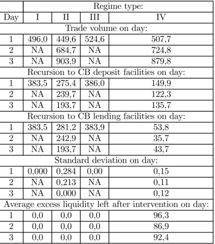
This section contains the results of the simulations for regime without reserve requirement. In practice, countries that applied these type of regime have also committed to frequent liquidity supplying injections to counter for the liquidity shocks. Since there is no deficiency that needs to be covered, the only purpose the funds serve is to secure commercial banks from incoming late liquidity shocks, that cannot be oﬀset by the interbank market. In the previous section, the asset value of the commercial bank sector was set just to make for the reserve requirement. To keep the results comparable, this time is just set to zero.

Before moving forward note that with daily OMO the optimal policy coincides with zero-excess liquidity, hence the results from regime I. and III. are identical.

Regime type:

Day I II III IV

Trade volume on day: 1 496,0 449,6 524,6 507,7 2 NA 684,7 NA 724,8 3 NA 903,9 NA 879,8

Recursion to CB deposit facilities on day: 1 383,5 275,4 386,0 149,9 2 NA 239,7 NA 122,3 3 NA 193,7 NA 135,7

Recursion to CB lending facilities on day: 1 383,5 281,2 383,9 53,8 2 NA 242,9 NA 35,7 3 NA 193,7 NA 43,7

Standard deviation on day: 1 0,000 0,284 0,00 0,15 2 NA 0,213 NA 0,11 3 NA 0,000 NA 0,12

Average excess liquidity left after intervention on day: 1 0,0 0,0 0,0 96,3

2 0,0 0,0 0,0 86,9 3 0,0 0,0 0,0 92,4

Table 2. No reserve requirement

The volume of trade is in general lower than in corresponding cases with the reserve requirement regime, but this just reflects the fact that without maintenance period this turns to be one-period model, hence the assets variance decreases. The market still works eﬃciently, with the end-of-trade banks liquidity (sum of initial assets, shock realisation and interbank borrowing) close to zero.

Limited liquidity on the market is transferred to the extend the standing facilities are used. Now that there is no cushion from funds kept the reserve

(29)

requirement, and most banks ending the trade with zero balance, they must rely on the central bank to oﬀset their late liquidity shock. Periodic OMO do not change that outcome significantly.

Without reserve requirement the rate responses very strongly to any changes in aggregate liquidity, but once it is exactly balanced, the volatility vanishes completely (the result already derived analytically in section 4.1). Increased sensitivity is due to the shape of demand curves (such as the ones on thefigure 2.) which are very elastic in the last day of the maintenance period. After aggregation, it transforms even relatively small liquidity shortage into large deviation from the target, a result that was observed by all researchers in the field. Zero variance with no excess funds follows just the logic of the base model, and property (4.1), hence the results for the daily OMO and last day of periodic regime.

Finally the last look on the value of liquidity if the OMO are performed on a periodic basis. It seems that in that case, most eﬀective policy would on average supply at least some liquidity, which reduces the use of lending facilities. It does not however improve the volatility of the rates which remains at high level.

To conclude the most important findings is that the zero-excess liquidity drives the rates variance to zero, but any excess (or shortage) of funds results in much higher volatility and use of standing facilities, compared to reserve requirement regime. It also leads to higher level of late intervention (in form of standing facilities or alternatively fine-tuning operations) with the market left without any liquidity buﬀer to oﬀset late shocks.

5.4

Diﬀerent maintenance period dates

This section contain the analysis of a regime where the banks are still obliged to satisfy reserve requirement, but the maintenance period for different banks (or group of banks) ends at different days. In our model, there are three maintenance period dates with 3 different banks groups. The total size of the market remained unchanged, hence each group is the size of 1/3 of the total number of banks. The value of assets (hence market liquidity) is kept at the same level as in the simulation with regular maintenance period, so it is just enough to satisfy individual bank deficiency.

The results of simulation seem to indicate that the banking sector is no more eager to trade than in the setups analysed so far. In fact in case of daily OMO the volume is even smaller. At the same time the, the optimal OMO value stays close to zero, indicating no excess liquidity. This gives support to the line of discussion from the paragraph 3.2.3. It is not optimal for the banks to ignore the reserve requirement completely, and count that they are going to satisfy it in the last period of its own maintenance period. Hence there is no ground for worries about banks overcoming reserve requirement whenever they are allowed for diﬀerent maintenance period dates.

(30)

Regime type:

Day I II III IV

Trade volume on day: 1 479,5 770,9 401,9 760,9 2 NA 907,1 NA 899,8 3 NA 953,7 NA 946,4

Recursion to CB deposit facilities on day: 1 117,2 157,5 93,7 126,4 2 NA 266,9 NA 214,5 3 NA 319,9 NA 268,3

Recursion to CB lending facilities on day: 1 97,6 127,8 101,6 125,3 2 NA 245,4 NA 243,6 3 NA 305,8 NA 302,5

Standard deviation on day: 1 0,134 0,192 0,009 0,092 2 NA 0,206 NA 0,086 3 NA 0,201 NA 0,114

Average excess liquidity left after intervention on day: 1 0,0 0,0 -1,5 -34,4

2 0,0 0,0 0,0 -48,3 3 0,0 0,0 0,0 -40,0

Table 3. Diﬀerent maintenance periods

So what is the eﬀectiveness of this operational policy as measured by the use of standing facilities and volatility of interest rates?

The first observation is that the spikes or regular patterns in the interest rates behaviour are gone. Little fluctuations in the standing facilities usage, present only in the regime with periodic open market operations are due to increased variance of assets between allotment dates.

The second observation is that how eﬀective this regime is (comparing to traditional reserve requirement) depends much on the frequency of the open market operations. In case of daily OMO the variance of the interest rates drops almost to the lowest level observed usually in maintenance period. It is not so clear with periodic OMO regimes, (especially for the case where optimisation algorithm is used) but the same general trend exists. It can be therefore concluded that introduction of diﬀerent maintenance period ending dates leads to significant reduction of the periodic spikes in volatility, at the same time keeping average level at relatively low level.

The analysis of the usage of standing facilities does lead to a similar conclusions. First of all, remember that only 1/3 of the number of banks used

in previous simulations now ends the maintenance period at the same day. Comparing to the situation where most of the facilities were used in the last period, it is no wonder significant improvement can be made. Once again using the optimisation algorithm helps to improve the results even further.

(31)

To summarise the results of that section, first the concerns about banks using diﬀerent maintenance dates system as a tool to trade liquidity between themselves seem to be misplaced. No increase in trade volume or permanently change aggregate liquidity is needed. When analysing the rates volatility the system works eﬃciently in case of daily OMO and although the results for periodic OMO, they point to the same direction.

5.5

Summary of results

The above sections contain the results for market volatility resulting from diﬀerent policy setups. It is not the goal of the study to decide in favour of any of them, yet a short comparison might be an interesting exercise.

The trade-oﬀbetween frequency of liquidity supply operations and stability of interest rates has been acknowledged in the literature. The results from that simulations seem to confirm that intuition. Indeed, the lowest volatility (actually -no volatility) is enjoyed by the regime without reserve requirement or other market frictions, with perfect forecasts of incoming liquidity shock and the Central Bank eager to supply massive amounts of liquidity both in early (OMO) and late (standing facilities) stage.

A bit more realistic scenario, also with very good results involves averaging provision and daily OMO. Apart from obvious technical diﬃculties from daily operations, it involves also shifting huge amounts of liquidity between diﬀerent days.

Allowing banks for diﬀerent maintenance period dates, succeeds in removing the spikes or periodic patterns from the data, but requires more late intervention during all days instead of the last one only.

There is one common point in all that regimes, a very important result of that study: even a relatively simple optimisation algorithm indicates that even though the aggregate liquidity matters, at least as much important is the distribution of liquidity among the banks. The same banking sector assets value might require diﬀerent policies in order to set the rates on target.

6 Conclusions

This paper uses simulation studies to compare the behaviour of the interbank market and CB interventions in diﬀerent structural setups. The starting point is the model for demand for the funds, based on the construction of Pérez-Quirós and Rodríguez-Mendizábal (2001). They analyse the regular patterns of the interest rate that can be observed in countries using averaging provision reserve requirement and channel system of standing facilities. The supply side of the market is given by the Central Bank open market operations, aiming for setting the interbank rates at some target.

The most importantfindings of the paper are that targeting the aggregate instead of individual bank liquidity is not enough to maintain a low level of market volatility. Indeed the optimisation algorithm, which calculates the

(32)

optimal allotment taking into account individual information performs much better than simple policy keeping the market with no excess (or shortage) liquidity.

Apart from that, the popular view that frequent liquidity supplying operations result in lower variance also finds support here. Zero variance is possible only under the unrealistic scenario where the central bank can predict the autonomous liquidity factors with 100% probability and there is no reserve requirement. In that case however the burden of oﬀsetting the late liquidity shock is totally on the standing facilities, with the interbank market left with no liquidity. Some specific features of the money markets such as the volatility increased toward the end of the maintenance with the averaging provision regime are replicated here as well. Introducing diﬀerent maintenance period dates as a new type of regime helps to reduce the periodic spikes, but results in higher use of standing facilities.

Analysing different setups offers an interesting comparison of costs and benefits of the policies applied by different Central Banks, but does not attempt to evaluate what is the optimal policy for a given country. Answering that question requires an estimate of how costly the liquidity supplying operations are for central authorities in different countries and what are the determinants of that cost.

(33)

References

Bartolini, L — Bertola, G — Prati, A (2001) Bank’s reserve management, transaction costs, and the timing of federal reserve intervention. Journal of Banking and Finance 25 (7), 1287—1317.

Bartolini, L — Bertola, G — Prati, A (2002) Day-to-day monetary policy and the volatility of the federal funds rate. Journal of Money, Credit and Banking, 34 (1), 137—159.

Bartolini, L — Prati, A (2003) Cross-country diﬀerences in monetary policy execution and money market rates’ volatility.StaﬀReports 175, Federal Reserve Bank of New York.

Bindseil, U (2004) Monetary Policy Implementation. Theory — Past — Present.Oxford University Press.

Cox, A H — Leach, R F (1964) Defensive open market operations and the reserve settlement periods of member banks.Journal of Finance 19 (1), 76—93.

Gaspar, V — Pérez-Quirós, G — Rodríguez-Mendizábal, H (2004) Interest rate determination in the interbank market.Working paper series 351, European Central Bank.

Hamilton, J D (1996)The daily market for federal funds.The Journal of Political Economy 104 (1), 26—56.

Moschitz, J (2004) The determinants of the overnight interest rate in the euro area. Working Paper Series 393, European Central Bank.

Pérez-Quirós, G — Rodríguez-Mendizábal, H (2001) The daily market for funds in europe: what has changed with the emu. Working paper series 67, European Central Bank.

Poole, W (1968)Commercial bank reserve management in a stochastic model: implications for monetary policy. Journal of Finance 23 (5), 769—791.

Välimäki, T (2003)Fixed rate tenders and the overnight money market equilibrium.Ph.D. thesis, Helsinki School of Economics and Bank of Finland.

(34)

Appendix A

Proof the results from section 3.1

The expected profit maximisation problem of a bank can be written as

max bt Et(Πi) = max bt Et(itbt−ct) (A1.1) where E(ct) = il ∙Z −mt+bt−θt−ε1t −∞ (mt−bt+θt+εt)f(ε2t)dε2t ¸ − (A1.2) id ∙Z _∞ −mt+bt−θt−ε1t (mt−bt+θt+εt)f(ε2t)dε2t ¸

The expected profit function can be then rewritten as

Et(Πt) = itbt−il(mt−bt+θt+ε1t)F (−mt+bt−θt−ε1t) +id(mt−bt+θt+ε1t) (1−F (−mt+bt−θt−ε1t)) −il ∙Z −mt+bt−θt−ε1t −∞ ε2tf(ε2t)dε2t ¸ (A1.3) +id ∙Z _∞ −mt+bt−θt−ε1t ε2tf(ε2t)dε2t ¸

The first order conditions for that problem with respect to bt are

−it = ilF (−mt+bt−θt−ε1t)−il(mt−bt+θt+ε1t)f(−mt+bt−θt−ε1t)

−id(1₋F (₋mt+bt−θt−ε1t))

−id(mt−bt+θt+ε1t)f(−mt+bt−θt−ε1t) (A1.4)

+il(mt−bt+θt+ε1t)f(−mt+bt−θt−ε1t)

+id(mt−bt+θt+ε1t)f(−mt+bt−θt−ε1t)

where the last line follows from Leibniz rule. Rearranging yields

it=ilF (−mt+bt−θt−ε1t) +id(1−F (−mt+bt−θt−ε1t)) (A1.5)

(35)

Appendix B

Simulation method

B.1 The demand side

I start with the basic case with reserve requirement and 3-day maintenance period (T) In the first period each bank decides about the value of optimal borrowing level based on a) current interest rate b) its own liquidity and c) expectations about future rates. The last element is necessary to calculate the derivatives of the value function and I will assume they will be equal to CB target rate. Using traditional grid method it is possible to calculate the value functions in all possible states in period T (last day). By substituting these values into eq. (3.9) one can compute analogous derivatives in period T ₋1 and finally use them to calculate the optimal borrowing for some initial guess of the interest rates at T₋2. The same procedure is repeated for allN banks to come up with the aggregate borrowing until the market clearing condition is satisfied, or no further improvement can be made.

Once the interest rate and optimal borrowing for each bank participant in

T ₋2 are known. I can move to following periods T ₋1 and T. Each time shock realisations move the system to new states (ie assets and deficiency) for which above procedure is repeated.

The behaviour of the interbank system without reserve requirements replicates simply the last stage of the procedure above, using diﬀerent parameters of the monetary policy (such as narrow borders of the channel system).

Finally in the last regime, banks have diﬀerent maintenance periods. To capture that I have created three groups of banks, n banks in each, that share common end of maintenance period date. The n is set in a way so the total number of banks is similar in all setups. Then, given market rate one can compute the individual demands for each group members, using the procedure already described above. The resulting rate satisfies market clearing conditions. After the rate and the lending is calculated, I use them to come up with a next day deficiencies (except of course for the group that starts new maintenance period, in which case they are reset to the initial values) and assets. To ensure that these results are comparable with other setups (where I had only 3 periods) I reset the asset value of all banks every 3rd iteration (otherwise assets value following random walk are becoming more volatile with each round of the simulation).

B.2 The supply side

The value of cenral bank allotment is detrmined in two diﬀerent ways. One — called here zero-excess liquidity — just supplied the value of funds equal to the sum of autonomous liquidity factors, so the market is left with neutral liquidity. A second way is to use a simple optimisation algorithm, that takes some value of allotment, checks what are predicted interest rates and if any improvement can be made by changing liquidity value. Once the decision has

(36)

been made about the optimal allotment value, it is distributed evenly among market participants.

Analysing the supply policy, note that between OMO and the opening of interbank market, another shock realisation occurs (denotedε1t in the paper)

meaning, that the rate that is calculated in the optimisation alrorithm and

final end-of-the-day rate are going to be diﬀerent, if only the distribution of shocks matters (which is thefinding of the paper).

The parameters of the simulation are set so the model is comparable with earlier research. Increasing the shock variance or decreasing market assets results in higher rates volatility, but the results are generally robust.

(37)

BANK OF FINLAND RESEARCH DISCUSSION PAPERS

ISSN 0785-3572, print; ISSN 1456-6184, online

1/2006 Juha-Pekka Niinimäki – Tuomas Takalo – Klaus Kultti The role of comparing in financial markets with hidden information. 2006. 37 p.

ISBN 952-462-256-4, print; ISBN 952-462-257-2, online.

2/2006 Pierre Siklos – Martin Bohl Policy words and policy deeds: the ECB and the euro. 2006. 44 p. ISBN 952-462-258-0, print; ISBN 952-462-259-9, online. 3/2006 Iftekhar Hasan – Cristiano Zazzara Pricing risky bank loans in the new

Basel II environment. 2006. 46 p. ISBN 952-462-260-2, print; ISBN 952-462-261-0, online.

4/2006 Juha Kilponen – Kai Leitemo Robustness in monetary policymaking: a case for the Friedman rule. 2006. 19 p. ISBN 952-462-262-9, print;

ISBN 952-462-263-7, online.

5/2006 Juha Kilponen – Antti Ripatti Labour and product market competition in a small open economy – Simulation results using the DGE model of the Finnish economy. 2006. 51 p. ISBN 952-462-264-5, print;

ISBN 952-462-265-3, online.

6/2006 Mikael Bask Announcement effects on exchange rate movements: continuity as a selection criterion among the REE. 2006. 43 p. ISBN 952-462-270-X, print; ISBN 952-462-271-8, online.

7/2006 Mikael Bask Adaptive learning in an expectational difference equation with several lags: selecting among learnable REE. 2006. 33 p.

ISBN 952-462-272-6, print; ISBN 952-462-273-4, online.

8/2006 Mikael Bask Exchange rate volatility without the contrivance of fundamentals and the failure of PPP. 2006. 17 p. ISBN 952-462-274-2, print; ISBN 952-462-275-0, online.

9/2006 Mikael Bask – Tung Liu – Anna Widerberg The stability of electricity prices: estimation and inference of the Lyapunov exponents. 2006. 19 p.

ISBN 952-462 276-9, print; ISBN 952-462- 277-7, online.

10/2006 Mikael Bask – Jarko Fidrmuc Fundamentals and technical trading: behavior of exchange rates in the CEECs. 2006. 20 p.

(38)

11/2006 Markku Lanne – Timo Vesala The effect of a transaction tax on exchange rate volatility. 2006. 20 p. ISBN 952-462-280-7, print;

ISBN 952-462-281-5, online.

12/2006 Juuso Vanhala Labour taxation and shock propagation in a New Keynesian model with search frictions. 2006. 38 p. ISBN 952-462-282-3, print;

ISBN 952-462-283-1, online.

13/2006 Michal Kempa Money market volatility – A simulation study. 2006. 36 p. ISBN 952-462-284-X, print; ISBN 952-462-285-8, online.

(39)

Suomen Pankki Bank of Finland P.O.Box 160

FI-00101

HELSINKI

Money market volatility, A simulation study

Michal Kempa

Money market volatility – A simulation study

Simulointitutkimus rahamarkkinoiden

Contents

1 Background and motivation...7

6 Conclusions ...29

1 Introduction

2 Model overview

3 Demand side

Reserve requirement

4 Supply side

No reserve requirement

Reserve requirement

5 Simulation study

Method outline

Averaging reserve requirement

No reserve requirement

Diﬀerent maintenance period dates

Summary of results

6 Conclusions

References

Appendix A

Appendix B

BANK OF FINLAND RESEARCH DISCUSSION PAPERS