Quasi Monte Carlo and multilevel Monte Carlo methods for computing posterior expectations in elliptic inverse problems

warwick.ac.uk/lib-publications

Scheichl, R., Stuart, A. M. and Teckentrup, A. L.. (2017) Quasi-Monte Carlo and multilevel Monte Carlo methods for computing posterior expectations in elliptic inverse problems. SIAM/ASA Journal on Uncertainty Quantification, 5 (1). pp. 493-518.

Permanent WRAP URL:

http://wrap.warwick.ac.uk/96053

Copyright and reuse:

The Warwick Research Archive Portal (WRAP) makes this work of researchers of the University of Warwick available open access under the following conditions. Copyright © and all moral rights to the version of the paper presented here belong to the individual author(s) and/or other copyright owners. To the extent reasonable and practicable the material made available in WRAP has been checked for eligibility before being made available.

Copies of full items can be used for personal research or study, educational, or not-for-profit purposes without prior permission or charge. Provided that the authors, title and full bibliographic details are credited, a hyperlink and/or URL is given for the original metadata page and the content is not changed in any way.

Publisher’s statement:

First Published in SIAM/ASA Journal on Uncertainty Quantification in 5 (1), 2017 published by the Society for Industrial and Applied Mathematics (SIAM). Copyright © by SIAM. Unauthorized reproduction of this article is prohibited.

A note on versions:

The version presented in WRAP is the published version or, version of record, and may be cited as it appears here.

arXiv:1602.04704v2 [math.NA] 2 Mar 2017

Quasi-Monte Carlo and Multilevel Monte Carlo Methods for

Computing Posterior Expectations in Elliptic Inverse Problems

R. Scheichl, A.M. Stuart, A.L. Teckentrup

Abstract

We are interested in computing the expectation of a functional of a PDE solution under a Bayesian posterior distribution. Using Bayes’ rule, we reduce the problem to estimating the ratio of two related prior expectations. For a model elliptic problem, we provide a full convergence and complexity analysis of the ratio estimator in the case where Monte Carlo, quasi-Monte Carlo or multilevel Monte Carlo methods are used as estimators for the two prior expectations. We show that the computational complexity of the ratio estimator to achieve a given accuracy is the same as the corresponding complexity of the individual estimators for the numerator and the denominator. We also include numerical simulations, in the context of the model elliptic problem, which demonstrate the effectiveness of the approach.

1

Introduction

Simulation frequently plays an essential role in the mathematical modelling of physical processes. However, the model parameters are often subject to uncertainty. This may be due to incomplete or inaccurate knowledge of the system or due to an inherent variability. It is important to understand how this uncertainty in the input parameters influences the reliability of the simulation outputs.

In the Bayesian framework, we initially assign a probability distribution, called the prior dis-tribution, to the input parameters. In addition observations, related to the model outputs, are often available, and it is then possible to reduce the overall uncertainty and get a better repre-sentation of the input parameters by conditioning the prior distribution on this data. This leads to the posterior distribution on the input parameters. The goal of the simulations is then often to compute the expected value of a quantity of interest (related to the model outputs) under the posterior distribution. This is the problem of Bayesian inference.

Typically, the posterior distribution is intractable, in the sense that direct sampling is unavail-able. One way to circumvent this problem is to use a Markov chain Monte Carlo (MCMC) approach to sample from the posterior distribution [40, 18, 11, 32, 9]. However, for large-scale applications where the number of input parameters is typically large and the solution of the forward model expensive, MCMC methods require careful tuning and may become infeasible in practice.

expectations, which are also well-suited to the case of high dimensional inputs. In particular, we investigate the use of Monte Carlo (MC), quasi-Monte Carlo (QMC) [38, 37, 35, 26] and multilevel Monte Carlo (MLMC) [25, 30, 2, 47, 29, 20] methods. The work is closely related to the inde-pendent works [14, 15, 23] that also investigate the use of QMC methods in computing posterior expectations. The papers [14, 15] are narrower in the range of problems considered. Their analysis is based on holomorphy arguments which require uniformly bounded coefficients, thus excluding the Gaussian case considered here. On the other hand, the range of methods considered is wider and includes higher-order QMC and multilevel QMC methods. The work [23] investigates the use of higher order QMC methods for computing posterior expectations arising from partial differential equations posed on random domains, again in the case of bounded parameters.

As a particular example, we consider the model inverse problem of determining the distribution of the diffusion coefficient of a divergence form elliptic partial differential equation (PDE) from ob-servations of a finite set of noisy continuous functionals of the solution. The coefficient distribution is assumed to be determined by an infinite number of scalar parameters through a basis expan-sion. In contrast to the works [44, 41, 43, 14], our analysis includes also results in the technically demanding case of log-normal diffusion coefficients, where the differential operator depends in a non-affine way on the parameters, each of which is modelled as a Gaussian random variable under the prior distribution. We provide a full convergence and complexity analysis of the estimator of the posterior expectation in the case of MC, QMC and MLMC sampling. We also demonstrate the effectiveness of this approach for the estimation of a typical quantity of interest derived from the elliptic inverse problem. The main conclusion of our work is that, for a given accuracy, the cost of computing the posterior expectation with any of these Monte Carlo variants is proportional to the computational complexity of the same estimator for prior expectations.

The remainder of this paper is organised as follows. Section 2 provides the mathematical set-up of the inverse problem of interest, including the formulation of ratio estimators for posterior ex-pectations. Section 3 is then devoted to the analysis of the error committed by approximating the governing equations by finite elements, and Section 4 introduces MC, QMC and MLMC estimators together with bounds on their sampling errors, extending the QMC analysis to non-linear function-als. In Section 5, we then provide a full convergence and complexity analysis of ratio estimators of posterior expectations. We demonstrate the performance of the proposed ratio estimators on a specific quantity of interest in Section 6, and finally provide some conclusions in Section 7.

2

Bayesian Inverse Problems

Let X and V be separable Banach spaces, and define the Borel measurable mappings _G :X _→ V and _H : V _→ Rm_{, for some m ∈} N_{. We will refer to G as the forward map and to H as the}

observation operator. We denote by F : X → Rm _{the composition of H and G, and by | · | the}

Euclidean norm on Rm_{. The inverse problem of interest is to determine the unknown function}

u_∈X from the noisyobservations (ordata) y_∈Rm _{given by}

y =_H(_G(u)) +η, (2.1)

where the noise η is a realisation of the Rm_{-valued Gaussian random variable N(0,Γ), for some}

(known) covariance matrix Γ. For simplicity, we will assume that Γ = σ2_ηI, for some positive constant σ2

We adopt a Bayesian perspective in which, in the absence of data, uis distributed according to a prior measureµ0. Under the conditions given in Proposition 2.1 below, the posterior distribution

µy on the conditioned random variable u|y is absolutely continuous with respect to µ0 and given

by an infinite dimensional version of Bayes’ Theorem. This takes the form

dµy dµ0

(u) = 1

Zθ(G(u)), (2.2)

where

θ(ζ) = exp[−Φ(ζ)], Φ(ζ) = 1 2σ2

η

|y− H(ζ)|2 and Z =E_µ

0[θ(G(u))]. (2.3)

The following proposition from [45] provides conditions under which the posterior distribution µy

is well defined and satisfies (2.2).

Proposition 2.1. Assume the map _F :X_→Rm _{is continuous andµ0(X) = 1.Then the posterior}

distributionµy _{is absolutely continuous with respect the prior distributionµ}

0, with Radon-Nikodym

derivative given by (2.2).

In applications, it is often of interest to compute the expectation of a functional φ:V _→R _of

G(u) under the posterior distribution µy. If we define

ψ(ζ) =θ(ζ)φ(ζ) and Q=E_{µ0[ψ(G(u))], (2.4)}

it follows from (2.2) that the posterior expectation ofφ(G(u)) can be written as

E_µy[φ(G(u))] =

E_µ

0[ψ(G(u))]

E_{µ0[θ(G(u))]} =

Q

Z. (2.5)

We will approximate E_µy[φ(G(u))] by using different Monte Carlo type methods to compute the prior expectations Z and Q.

2.1 Parametrisation of the Unknown Input

We consider the setting where the Banach space X is a space of real-valued functions defined on a bounded spatial domain D _⊂ Rd, for some dimension d = 1,2 or 3. For ease of presentation, we shall restrict our attention to the caseX =C(D), the space of continuous functions onD, but other choices are possible (cf. Remark 2.12), as is the extension to vector-valued functions.

We assume that the unknown function u∈X admits a parametric representation of the form

u(x) =m0(x) + ∞

X

j=1

ujφj(x), (2.6)

where m0 ∈ X, {φj}∞j=1 denotes an infinite sequence in X (typically normalised to one in X or

in a larger space containing X) and _{uj}∞j=1 ⊂ R∞ denotes a set of real-valued coefficients. By

randomising the coefficients _{uj}∞j=1, we create real-valued random functions on D. To this end,

we introduce the deterministic, monotonically non-increasing sequence γ = {γj}∞_j=1 and the i.i.d

random sequence ξ ={ξj}∞j=1, and set uj =γjξj. To emphasise the dependence of u onξ, we will

write u=u(x;ξ).

2.1.1 Uniform Priors

In the case of uniform priors, we specify the i.i.d. sequence of random variables ξ = _{ξj}∞j=1 by

choosing ξj ∼U[−1,1], a uniform random variable on [−1,1], and the deterministic sequence γ is

chosen absolutely summable, γ ∈ ℓ1(R∞_{). The functions {φj}}∞

j=1 and m0 are chosen as elements

of C(D), and are assumed normalised so thatkφjk_C(D)= 1, for allj∈N.

We then have the following result from [12].

Lemma 2.2. Suppose there are finite, strictly positive constantsmmin, mmax and r such that

min

x∈D

m0(x) ≥ mmin, max

x∈D

m0(x) ≤ mmax and kγkℓ1 = r

1 +rmmin.

Then the following holds almost surely: the function u(·;ξ)defined in (2.6)is in C(D)and satisfies the bounds

1

1 +rmmin ≤u(x;ξ)≤mmax+ r

1 +rmmin, for almost all x∈D.

Note in particular that the upper and lower bounds on u in Lemma 2.2 are independent of the particular realisation of the random sequence ξ. WithX=C(D), it follows from Lemma 2.2 that µ0(X) = 1. We furthermore have the following result from [12] on the spatial regularity of the

functionu in the case where the functions (m0,{φj}∞j=1) are H¨older continuous.

Lemma 2.3. Suppose m0 and {φj}j≥1, are in Cα(D), the space of H¨older continuous functions

with exponent α _≤ 1, and suppose P∞_j=1|γj|2kφjkβ_Cα_(D) < ∞, for some β ∈ (0,2). Then the functionu(_·;ξ) defined in (2.6)is in Ct(D) almost surely, for any t < αβ/2.

2.1.2 Gaussian Priors

For Gaussian priors, we specify the i.i.d sequence of random variables ξ by choosing ξj ∼N(0,1),

a standard Gaussian random variable with mean 0 and variance 1. We choose the sequences {φj}∞j=1and{γj2}∞j=1to be the eigenfunctions and eigenvalues, respectively, of a covariance operator

C : L2(D) → L2(D), such that the series (2.6) is the Karhunen-Loeve (KL) expansion of the Gaussian measure µ0 = N(m0,C) on L2(D). Denote by c : D×D → R the covariance kernel

corresponding to the covariance operatorC. It follows from Mercer’s Theorem that the eigenvalues

{γ2_j}∞

j=1are positive and summable, and the equality c(x, y) =

P∞

j=1γj2φj(x)φj(y) holds for almost

all x, y_∈D.

We have the following result on the spatial regularity of the functionu from [4, 12].

Lemma 2.4. Let C denote the covariance operator with covariance kernel c satisfying c(x, y) = g(_kx ₋y_k), for all x, y _∈ D, some norm _{k · k} on Rd _{and some Lipschitz continuous function}

g∈C0,1(D). Let{φj}∞_j=1 and{γ_j2}∞_j=1 be the eigenfunctions and eigenvalues ofC, respectively, and

supposem0∈Ct(D), for somet <1/2. Then, the function u(·;ξ) defined in (2.6) is also inCt(D)

almost surely.

An example of a covariance kernel c(x, y) that satisfies the assumptions of Lemma 2.4 is the exponentialcovariance kernel

where the positive parametersσ2 and λare known as the variance and correlation length, respec-tively, and typically r= 1 or 2.

It follows from Lemma 2.4 that if the covariance operator C is smooth enough, so that the functiongis Lipschitz continuous, the functionu(_·;ξ) is almost surely continuous. WithX =C(D), it hence follows that µ0(X) = 1.

For practical applications, such as the problem described in Section 2.2, it is often of interest to construct a function that is strictly positive on D. For this reason, we consider the function a(_·;ξ) = exp[u(_·;ξ)]. Since u(_·;ξ) is almost surely continuous, we can define almost surely the quantities

amin(ξ) = min x∈D

a(x;ξ), and amax(ξ) = max x∈D

a(x;ξ).

We have the following result on the boundedness of the function a[4, 5].

Lemma 2.5. Let the assumptions of Lemma 2.4 hold. Then a(·;ξ) = exp(u(·;ξ)) is in Ct(D) almost surely, for any t <1/2. Furthermore,

0< amin(ξ)≤a(x;ξ)≤amax(ξ)<∞, for almost all x∈D andξ ∈R∞,

and a−_min1 _∈Lr(R∞_{), amax∈L}r₍R∞_{) and a∈L}r₍R∞_{, C}t_{(D)), for allr∈[1,∞).}

Other, smoother covariance kernels, such as theGaussian kernel

c(x, y) =σ2exp[_−kx₋y_k2₂/ λ2]

or the kernels from the Mat´ern family, also satisfy the assumptions of Lemmas 2.4 and 2.5, but they lead to a significantly higher spatial regularityt_≥1/2 of a.

2.1.3 Finite-dimensional approximation

In simulations, it is often necessary to use a finite-dimensional approximation of the unknown u. Given the parametrisation (2.6), this can be achieved by simply truncating the series at finite truncation order J, or through best N-term approximations [7, 48]. For simplicity, we here choose the former, and make the following assumption in the remainder of this paper.

Assumption A1. (Finite Truncation Order) Suppose the coefficients _{γj}∞_j=J+1 are all equal to

zero, for some finiteJ ∈N_{, such that}

u(x;ξ) =u(x;ξJ) =m0(x) + J

X

j=1

γjξjφj(x), (2.8)

whereξJ :={ξj}Jj=1∈RJ.

An important question is how one should optimally choose the truncation orderJ in (2.8), and the answer typically involves a trade-off between choosingJ sufficiently large to retain a required accuracy, and sufficiently small to avoid an unnecessarily large computational cost associated to sampling fromu. We will in this paper assume that J ∈N_{is given, and will not explicitly discuss}

how to chooseJ. We refer the interested reader to the works [4, 35, 47, 26].

The series (2.8) defines a linear mapping P : RJ _{→ X, with P(ξJ) = u, and we will define}

coefficient spaceRJ_{, equipped with the Borel productσ-algebra. For the uniform priors considered}

in section 2.1.1, the measureP is the product measure

P_{(dξJ) =}

J

Y

j=1

dξj

2 . (2.9)

For the Gaussian priors in section 2.1.2, we have

P_{(dξJ) =}

J

Y

j=1

1 √

2π exp[−ξ

2

j/2] dξj. (2.10)

Corollary 2.6. Suppose Assumption A1 holds. Then (i) Lemmas 2.2 and 2.3 hold; and (ii) if {φj}Jj=1 and {γj2}Jj=1 are chosen as the first J elements of {φj}∞j=1 and {γj2}∞j=1 in Lemma 2.4,

respectively, then Lemma 2.4 and 2.5 hold.

Proof. Part (i) follows directly from Lemmas 2.2 and 2.3, since the parametrisation (2.8) is just a special case of (2.6). Part (ii) is proven in [4].

Remark 2.7. (Alternative Approximations) The truncated parametrisation (2.8) is not the only way to obtain an approximation of u from which we can easily produce samples for simulation. In the case of Gaussian priors, knowledge of the covariance kernel c allows us to assemble the covariance matrix of the Gaussian vector [u(x1), u(x2), . . . , u(xn)], for anyn∈Nand{xi}ni=1⊆D,

and we can hence use methods based on factorisations of the covariance matrix, such as [17], to sample fromuat a finite number of locations in the domain D. In applications such as the elliptic problem discussed in section 2.2, this is usually sufficient, since typically quadrature methods are used to compute the numerical approximation discussed in section 3. For more details, we refer the interested reader to [27, 28, 46].

2.2 Model Elliptic Problem

We consider the model inverse problem of determining the distribution of the diffusion coefficient of a divergence form elliptic partial differential equation (PDE) from observations of a finite set of noisy continuous functionals of the solution. LetD⊂Rd_{, ford= 1,2 or 3, be a bounded Lipschitz}

domain, and denote by∂Dits boundary. The forward problem which underlies the inverse problem of interest here is to find the solution p(_·;ξJ) of the following linear elliptic PDE,

− ∇ ·(k(x;ξJ)∇p(x;ξJ)) =f(x) inD, p(·;ξJ) = 0 on ∂D, (2.11)

for given functions k(·;ξJ) ∈ C(D) and f ∈H−1(D). Although all results in this section apply

also in the case of infinite-dimensional parameter vectors ξ, we restrict our attention to finite-dimensionalξJ for consistency.

The variational formulation of (2.11) is to find p(·;ξJ)∈H01(D) such that

b(p, q;ξJ) =L(q), for allq ∈H01(D), (2.12)

where the bilinear formband the linear functional Lare defined as usual, for all v, w∈H₀1(D) by

b(v, w;ξJ) =

Z

D

k(x;ξJ)∇v(x)· ∇w(x) dx and L(w) =hf, wiH−₁ (D),H1

We say that p(_·;ξJ) is a weak solution to (2.11) iff p(·;ξJ)∈H01(D) and p(·;ξJ) satisfies (2.12).

In the inverse problem, we take the coefficientkto be a function of the unknownu, in which case both the coefficientkand the solutionpdepend on the random sequenceξJ. When the dependence

on ξJ of k and p is irrelevant, we will simply write k = k(x) and p = p(x). With the unknown

functionu(_·;ξJ) as in Section 2.1, we choose

• k(·;ξJ) =u(·;ξJ), in the case of the uniform priors described in Section 2.1.1, and

• k(_·;ξJ) = k∗+ exp(u(·;ξJ)), in the case of Gaussian priors, for some given continuous

non-negative function k∗≥0.

By Lemmas 2.2 and 2.5, both these choices ensure that the diffusion coefficientk(·;ξJ) in (2.12) is

strictly positive on D,P_{-almost surely. In terms of the notation in previous sections, the Banach}

space X is the space of continuous functions C(D) as before. The forward map G is defined by G(u) = p, i.e. it maps the unknown function u(·;ξJ) to the solution p(·;ξJ). (Note that the

definition of _G differs between the two choices k =u and k= k∗_{+ exp(u).) We take the Banach}

space V as the Sobolev space H₀1(D).

Existence and uniqueness of the weak solutionp(·;ξJ) is ensured by the Lax-Milgram Theorem.

As in previous sections, let kmin(ξJ) and kmax(ξJ) be such that

0< kmin(ξJ)≤k(x;ξJ)≤kmax(ξJ)<∞, for almost all x∈Dand for ξJ P-almost surely.

For uniform priors,kmin(ξJ) and kmax(ξJ) are independent of ξJ. If k∗(x) >0, for allx∈D, then

kmin(ξJ) is also independent ofξJ in the Gaussian case.

Definition 2.8. We will refer to the coefficient k as uniformly elliptic (respectively uniformly bounded) when kmin(ξJ) (respectivelykmax(ξJ)) is independent ofξJ.

The following is a direct consequence of the Lax-Milgram Lemma and Lemmas 2.2 and 2.5.

Lemma 2.9. For P_{-almost all ξJ ∈} RJ_{, there exists a unique weak solution p(·;ξJ) ∈ H}1

0(D) to

the variational problem (2.12) and

p(·;ξJ)

_H1_(D) ≤

kfkH−1

(D)

kmin(ξJ)

.

Furthermore, p_∈LrP(RJ, H₀1(D)), for allr ∈[1,∞). Ifkis uniformly elliptic, then the result holds

also for r=_∞.

In order to conclude on the well-posedness of the posterior distributionµy, we furthermore have the following result on the continuity of the forward map_G.

Lemma 2.10. The map G:X→V, G(u) =p, is continuous.

Proof. Denote byp1 andp2 two weak solutions of (2.12) with the same right hand sidef and with

coefficients k1 and k2, respectively. Let kmin and kmax be such that

0< kmin≤ki(x)≤kmax<∞, for almost all x∈D,

fori= 1,2. Then it follows from the variational formulation (2.12) that

|p1−p2|H1_(D)≤ k

fkH−1 (D)

k2 min

In the case k = u, the continuity of _G now follows immediately. In the case k = exp(u), the continuity of _G follows from the continuity of the exponential function.

We then have the following corollary to Proposition 2.1, which follows immediately from Lemmas 2.2, 2.4 and 2.10, together with the continuity of the observation operatorH.

Corollary 2.11. For the forward map_G defined by_G(u) =p, the posterior measureµy _{is absolutely}

continuous with respect to the prior measure µ0, with Radon-Nikodym derivative (2.2).

Remark 2.12. (Piecewise continuous coefficients) Although we here restrict our attention to the case of continuous random coefficients, the theory extends to the piecewise continuous case where a further source of randomness can be introduced in the partitioning of the computational domain Dinto sub-domains. The well-posedness of the posterior distribution in this case was shown in [?]. The regularity and spatial discretisation error (as discussed in Section 3) were analysed in [47, 46].

3

Finite Element Discretisation

In this section, we analyse the error introduced in the computation of the prior expectationsZ and Qby a finite element approximation of the forward map_G. We consider only standard, continuous, piecewise linear finite elements on polygonal/polyhedral domains in detail. To this end, denote by {Th}h>0 a shape-regular family of simplicial triangulations of the Lipschitz polygonal/polyhedral

domainD, parametrised by their mesh width h:= maxτ∈Thdiam(τ). Associated with each trian-gulation Th we define the space

Vh :=qh ∈C(D) :qh|τ linear for all τ ∈ Th and qh|∂D = 0 (3.1)

of continuous, piecewise linear functions on Dthat vanish on the boundary∂D.

The finite element approximation to (2.12), denoted by ph, is now the unique function in Vh

that satisfies

b(ph, qh;ξJ) =L(qh), for allqh∈Vh, (3.2)

where the bilinear formband the functionalLare as in (2.13). Note that, in particular, this implies thatph satisfies the same bound as in Lemma 2.9:

|ph(·;ξJ)|H1_(D)≤ kfk_H−₁

(D)/kmin(ξJ). (3.3)

The approximate forward map Gh : X → V is then defined by Gh(u) = ph, and we denote the

resulting approximations of Z and Q, respectively, by

Zh=Eµ0[θ(Gh(u))] and Qh=Eµ0[ψ(Gh(u))].

A standard technique to prove convergence of finite element approximations of functionals is to use a duality argument, similar to the classic Aubin Nitsche trick used to prove optimal convergence rates for the L2 _{norm. In the context of the elliptic PDE (2.11) with random coefficients, this}

Let v, w _∈ H₀1(D). Given a functional F : H₀1(D) _→ R_{, we denote by DvF(w) its Fr´echet}

derivative atw, applied to v. With pand ph as before, we define

DvF(p, ph) =

Z 1

0

DvF(p+λ(ph−p)) dλ,

and _|DvF|(p, ph) =

Z 1

0 |

DvF(p+λ(ph−p))|dλ,

which in some sense are averaged derivatives ofF on the path fromp toph. Let us now define the

following dual problem: findz_∈H1

0(D) such that

b(q, z;ξJ) =DqF(p, ph), for allq∈H01(D). (3.4)

Denote the finite element approximation of the dual solution z by zh ∈ Vh. It then follows from

the Fundamental Theorem of Calculus, Galerkin orthogonality of the primal problem (2.12) and boundedness of the bilinear form bthat

|F(p)₋F(ph)|=|b(p−ph, z;ξJ)|=|b(p−ph, z−zh;ξJ)| ≤kmax(ξJ)|p−ph|H1_(D)|z−z_h|_H1_(D).

In order to prove convergence of the finite element error _|F(p)₋F(ph)|, it hence suffices to prove

convergence of _|p₋ph|H1_(D) and |z−z_h|_H1_(D). For our further analysis, we make the following assumption on the smoothness of the mapsφandH. Examples of functionals satisfying Assumption A2 are discussed in [47], and include linear functionals, powers of linear functionals and boundary fluxes.

Assumption A2. (Differentiability) Let φ and Hi,i = 1, . . . , m, be continuously Fr´echet

differ-entiable on the path _{p+λ(p₋ph)}λ∈[0,1], and suppose that there exist t∗∈[0,1], q∗ ∈[1,∞] and

Cφ, CH∈Lq∗P(RJ) such that f ∈Ht∗−1(D),

|Dvφ|(p, ph)≤Cφ(ξJ)kvkH1−t∗(D), and |DvHi|(p, ph)≤CH(ξJ)kvkH1−t∗(D),

for all v_∈H1

0(D) and almost allξJ ∈RJ.

Let now F = φ or F = _Hi, for some i ∈ {1, . . . , m}. To get well-posedness of the primal

problem (2.12) and the dual problem (3.4), as well as existence and uniqueness of the solutions p(·;ξJ) ∈ H01(D) and z(·;ξJ) ∈ H01(D), for almost all ξJ ∈ RJ, it is sufficient to assume that

Assumption A2 holds with t∗ = 0. However, in order to prove convergence of the finite element

approximations, it is necessary to require stronger spatial regularity of p and z, which requires Assumption A2 to hold for somet∗ >0. We have the following result from [5, 47]. The assumptions

on D being polygonal and convex are purely to simplify the presentation. Proposition 3.1 also holds for piecewise smooth or for non-convex domains, but typically with stronger restrictions on the range ofs.

Proposition 3.1. Let D be a Lipschitz polygonal, convex domain, let k ∈ Lr∗

P (RJ, Ct(D)) and

k_min−1 ∈ Lr∗

P (RJ), for some t∈ (0,1] and r∗ ∈ [1,∞], and let Assumption A2 hold with t∗ = t and

q∗ = r∗. Then, the solutions p and z of (2.12) and (3.4) are both in LrP(RJ, H1+s(D)), for any

We will now show that the functionals θ and ψ appearing in the prior expectations Z and Q, respectively, satisfy the bounds in Assumption A2 provided φ and _H satisfy Assumption A2, as well as the growth conditions in Assumption A3 below.

Assumption A3. (Boundedness) Suppose there are constants M1, M2 >0 and n1, n2 ∈N, such

that

|φ(v)_{| ≤}M1

1 +_|v_|n1

H1_(D)

and _|H(v)_{| ≤}M2

1 +_|v_|n2

H1_(D)

, for all v_∈H₀1(D). (3.5)

Recall the product and chain rules for Fr´echet derivatives for functionals F1, F2 :H01(D) →R

and a function f :R_→R_:

Dv(F1F2)(w) =F2(w)DvF1(w) +F1(w)DvF2(w) and Dv(f◦F1)(w) =DDvF1(w)f(F1(w)).

We then have the following result.

Lemma 3.2. Let Assumption A2 hold with t∗ ∈ [0,1] and q∗ ∈ [1,∞], and suppose Assumption

A3 holds. Then

|Dvθ|(p, ph)≤Cθ(ξJ)kvkH1−t∗(D), and |Dvψ|(p, ph)≤Cψ(ξJ)kvkH1−t∗(D),

for all v _∈ H₀1(D) and for ξJ P-almost surely, where Cθ(ξJ) and Cψ(ξJ) are in LrP(RJ), for all

r_∈[1, q∗) If k is uniformly elliptic, then the result holds also forr =q∗.

Proof. First, we use the chain rule and product rule for Fr´echet derivatives to obtain

Dvθ(w) =Dv exp

"

− 1

2σ2 η

m

X

i=1

(yi− Hi(w))2

#!

=₋θ(w) 1 σ2

η m

X

i=1

DvHi(w)(yi− Hi(w)).

Denoting pλ =p+λ(ph−p), we then have

|Dvθ|(p, ph) =

Z 1

0 |

Dvθ(pλ)|dλ≤

Z 1

0

θ(pλ)

1 σ2 η m X i=1

|DvHi(pλ)| |yi− Hi(pλ))|dλ.

By the definition of θin (2.3), we have θ(pλ)≤1, for all λ∈[0,1]. By Assumption A3, it follows

that

|yi− Hi(pλ))| ≤C(1 +|pλ|_Hn21_(D))≤C(1 +kfkn_H2−1_(D)k

−n2

min(ξJ)),

for some (generic) constant C independent of the mesh size h and random parameter ξJ. It then

follows that

|Dvθ|(p, ph)≤

C σ2 η

(1 +_kf_kn2

H−₁ (D)k

−n2

min(ξJ)) m

X

i=1

|DvHi|(p, ph).

WithCθ(ξJ) = m C_σ2

η (1 +kfk

n2

H−1_(D)k −n2

min(ξJ))CH(ξJ), it then follows from Assumption A2 that

|Dvθ|(p, ph)≤Cθ(ξJ)kvkH1−t∗(D).

Next, using the product rule for Fr´echet derivatives, together with the result just proved, we have

Dvψ(w) =θ(w)Dvφ(w)−φ(w)θ(w)

1 σ2 η m X i=1

Withpλ as before, it then follows that

|Dvψ|(p, ph) =

Z 1

0 |

Dvψ(pλ)|dλ

≤

Z 1

0

θ(pλ)

"

|Dvφ(pλ)|+φ(pλ)

1 σ2

η m

X

i=1

|DvHi(pλ)| |δi− Hi(pλ)|

#

dλ.

Nowθ(pλ)≤1, for all λ∈[0,1]. By Assumption A3, it follows that

|φ(pλ)| max

i∈{1,...,m}|yi− Hi(pλ))| ≤C(1 +|pλ| n2

H1_(D))2 ≤C(1 +kfk2n_H−21_(D)k −2n2

min (ξJ)),

for some (generic) constant C independent of the mesh size h and random parameter ξJ. It then

follows that

|Dvψ|(p, ph)≤ |Dvφ|(p, ph) +

C σ2 η

(1 +_kf_k2n2

H−₁ (D)k

−2n2

min (ξJ)) m

X

i=1

|DvHi|(p, ph).

WithCψ(ξJ) =Cφ(ξJ) +m C_σ2

η (1 +kfk

2n2

H−1_(D)k −2n2

min (ξJ))CH(ξJ), it then follows that

|Dvψ|(p, ph)≤Cψ(ξJ)kvkH1−t∗(D).

Finally, recall that by Lemmas 2.2 and 2.5, we havek−_min1 (ξJ)∈L∞P (RJ) ifkis uniformly elliptic,

and k−_min1 (ξJ) ∈ LqP(RJ), for any 1 ≤ q < ∞, otherwise. Hence, it follows from Assumption A2,

together with H¨older’s and Minkowski’s inequalities, thatCθ(ξJ) andCψ(ξJ) are inLrP(RJ), for all

r_∈[1, q∗). If kis uniformly elliptic, we can also set r=q∗.

Bounds on the finite element errors _|θ(p)₋θ(ph)|and |ψ(p)−ψ(ph)|now follow directly from

Proposition 3.1 and Lemma 3.2.

Theorem 3.3. Under the assumptions of Proposition 3.1 and Lemma 3.2 with t ∈ (0,1] and r∗ ∈[1,∞], we have

kθ(p)−θ(ph)kLr

P(RJ)≤Ck,f,θ,D h

2s_{, and kψ(p)−ψ(p} h)kLr

P(RJ)≤Ck,f,ψ,Dh

2s_,

for any s < t and r < r∗. The constants Ck,f,θ,D andCk,f,ψ,D are independent ofh. Ifr∗=∞, we

can also bound the L∞

P norms. If t= 1, we can set s= 1.

Proposition 3.1, Lemma 3.2 and Theorem 3.3 hold, without any additional assumptions, also for infinite-dimensional parameter vectorsξ ∈R∞ _{[5, 47].}

4

Sampling methods

In this section, we briefly recall the main ideas behind Monte Carlo (MC), Multilevel Monte Carlo (MLMC) and quasi-Monte Carlo (QMC) estimators to compute the prior expectation Qh=

E_µ

4.1 Monte Carlo estimators

The standard Monte Carlo estimator forQh is

b

QMC_h,N = 1 N

N

X

i=1

ψ(ph(·;ξ_J(i))), (4.1)

whereξ_J(i)is theith sample ofξJ from the distributionP, andN independent samples are computed

in total. The estimator (4.1) is an unbiased estimator of Qh, with variance

V_[QbM C

h,N] =

V_[ψ(ph)]

N . (4.2)

4.2 Multilevel Monte Carlo estimators

The main idea of multilevel Monte Carlo estimation is simple. Linearity of the expectation operator implies that

E_µ0[ψ(ph)] =Eµ0[ψ(ph0)] +

L

X

ℓ=1

E_µ0[ψ(phℓ)−ψ(phℓ−₁)],

where_{hℓ}Lℓ=0are the mesh widths of a sequence of increasingly fine triangulationsThℓwithhL=h, the finest mesh width, andk1 ≤hℓ−1/hℓ ≤k2, for allℓ= 1, . . . , Land some 1< k1 ≤k2 <∞. The

multilevel idea is now to estimate each of the terms independently using a Monte Carlo estimator. Setting for convenience Y₀ψ =ψ(ph0), and Y

ψ

ℓ =ψ(phℓ)−ψ(phℓ−1), for ℓ= 1, . . . , L, we define the

MLMC estimator as

b

QML_h,{N ℓ} =

L

X

ℓ=0

b

Y_ℓ,Nψ,MC

ℓ =

L

X

ℓ=0

1 Nℓ

Nℓ

X

i=1

Y_ℓψ(·;ξ_J(i,ℓ)), (4.3)

where importantly the quantity Y_ℓψ(_·;ξ_J(i,ℓ)) uses the same sample ξ_J(i,ℓ) on both meshes. The estimator (4.3) is an unbiased estimator of Qh, with variance

V_[QbML

h,{Nℓ}] =

L

X

ℓ=0

V_[Yψ

ℓ ]

Nℓ ≤

C

L

X

ℓ=0

h4s_ℓ Nℓ

, (4.4)

where the last inequality follows from Theorem 3.3, with a constantC independent of _{hℓ}Lℓ=0 and

with 0_≤s < t_≤1, as defined in Proposition 3.1.

When defining the MLMC estimator (4.3), one can in fact also use level-dependent truncation levels Jℓ. This approach was analysed in [47], and can lead to further significant gains in terms of

computational cost.

4.3 Quasi-Monte Carlo estimators

Quasi-Monte Carlo methods are classically formulated as quadrature rules over the unit cube [0,1]J, for some J _∈ N_{. Treating ξJ as a deterministic parameter vector distributed according to the}

product uniform or Gaussian measure, respectively,

E_µ

0[ψ(ph)] =

Z

[0,1]J

whereξJ = Φ−_J1(v) denotes the inverse cumulative normal applied to each entry ofvin the Gaussian

case. In the uniform case, Φ−_J1 is the simple change of variables mappingvj to 2vj−1. We will use

a randomly shifted lattice rule to approximate the integral (4.5). This takes the form

b

QQMC_h,N = 1 N

N

X

i=1

ψph ·; ˜ξJ(i)

, where ˜ξ_J(i):= Φ−_J1

fraciz

N + ∆

, (4.6)

z ∈ {1, . . . , N −1}J _{is a generating vector, ∆ is a uniformly distributed random shift on [0,1]}J_,

and ”frac” denotes the fractional part function, applied component-wise. To ensure that every one-dimensional projection of the lattice rule has N distinct values we furthermore assume that each componentzj of zsatisfies gcd(zj, N) = 1 (cf. [16]).

The variance of the QMC estimator (4.6) is given by

V_[QbQMC

h,N ] =E∆[(Eµ0[ψ(ph)]−Qb

QMC

h,N )2]. (4.7)

To bound it, we make the following assumption on the integrandψ(ph).

Assumption A4. Letc1>0 be a constant independent of J and let bj :=γjkφjk_C0_(D), forj∈N. We assume that, for any multi-index ν ∈ {0,1}J with|ν|=P_j≤Jνj,

∂|ν|_ψ(p

h)

∂ξν

J

≤Ck,f,ψ,D

c|ν|

1 |ν|!

kmin(ξJ) J

Y

j=1

bνj

j .

For linear functionals ψ on H₀1(D), this has been proved in [35] and in [26] for the uniform and the Gaussian cases, respectively. In both cases, we can choose c1 = 1/ln 2. However, in the

Bayesian setting, both ψ and θ are inherently non-linear functionals of p. Nevertheless, if φ and H are linear functionals of p, and k is uniformly elliptic, Assumption A4 can be proved by using the classical Fa`a di Bruno formula [10], a multidimensional version of the chain rule. A proof for θ in the casem = 1 can be found in Appendix A. We omit the proof for ψ or form >1. A proof for general analytic functionals φand Hof p would be even more technical and require the use of generalisations of Fa`a di Bruno’s formula to Fr´echet derivatives. For this reason, we simply work under Assumption A4.

In the case of uniform priors, Assumption A4 was proven to hold in [14] using arguments from complex analysis and the holomorphy ofph as a function of ξJ.

Lemma 4.1. Suppose Assumption A4 holds and the sequence _{bj}∞j=1 is in lq(R∞), for some

q ∈(0,1]. Then, a randomly shifted lattice rule can be constructed via a component-by-component algorithm in_O(JNlogN) cost, such that

V_[QbQMC

h,N ]≤

Cψ,q,δN−1/δ, if q ∈(0,2/3],

Cψ,q N−(1/q−1/2), if q ∈(2/3,1),

for any δ ∈ (1/2,1], independently of J. For q = 1 and under further assumptions given in [26, Theorem 20] and [35, Theorem 6.4], we have V_[QbQMC

h,N ]≤CψN−1/2.

Proof. The proof follows those in [35, 26] with suitable changes to the product and order dependent (POD) weights if c1 6= 1/ln 2.

5

Mean Square Error and Computational Complexity

We will now use the results from Sections 3 and 4 to bound the mean square error (MSE) of estimators for the ratioQ/Z. To this end, let us denote byZbh andQbhone of the Monte Carlo type

estimators discussed in Section 4 forZh and Qh, respectively. Let us define the mean square error

eQbh

. b Zh 2 =E " Q Z − b Qh b Zh 2# . (5.1)

For MC and MLMC estimators, the expectation in the expression (5.1) above is with respect to the prior measureµ0 on X. For QMC estimators, it is with respect to the random shift ∆.

Rearranging the mean square error and using the triangle inequality, we have

eQbh

. b

Zh

2

= 1

Z2E

Q₋Qbh+ (Qbh/Zbh)

b

Zh−Z

2 ≤ 2 Z2 E h

(Qbh−Q)2

i

+ E

h

(Qbh/Zbh)2(Zbh−Z)2

i

. (5.2)

Our further analysis depends on the integrability of Qbh bZh, and we thus consider separately the

cases of uniformly and non-uniformly elliptic coefficients k.

5.1 Uniformly elliptic case

In the case where the coefficient k is uniformly elliptic, we have the following result on the in-tegrability of Qbh/Zbh. The assumptions on φ and H are more general than Assumption A3, and

allow for very general non-linear growth. Since, in general, Zb_h,ML_{N

ℓ} could be negative, we require stronger assumptions in the case of multilevel Monte Carlo estimators. In particular, we require the assumptions of Theorem 3.3 to hold with r =_∞, which means that the coefficient kneeds to be uniformly bounded as well as uniformly elliptic. The analysis of MLMC in Lemma 5.1 below therefore does not apply in the case of Gaussian priors.

Lemma 5.1. Suppose k is uniformly elliptic and there are two constants M1, M2>0, such that

|φ(v)_{| ≤}M1 and |H(v)| ≤M2, for all v∈H01(D) with |v|H1_(D)≤ kfk_H−1_(D)/kmin.

Then QbMC_h,N bZ_h,NMC _∈ L∞P (RJ), and Qb QMC h,N bZ

QMC

h,N ∈ L∞∆([0,1]J), with L∞-norms bounded

indepen-dently of h and N.

If in addition h0 is sufficiently small and the assumptions of Theorem 3.3 hold with r=∞, we

also have QbML_h,{N ℓ} bZ

ML h,{Nℓ} ∈L

∞

P (RJ), with L∞-norm bounded independently of {hℓ}, {Nℓ} and L.

Proof. Using the definition ofQbMC_h,N in (4.1), as well as the bound in (3.3) and the fact thatθ(v)≤1, for all v_∈H₀1(D), it follows that

|QbMC_h,N|=

1 N N X i=1

φ(ph(·;ξJ(i)))θ(ph(·;ξJ(i)))

and

b

Z_h,NMC= 1 N

N

X

i=1

θ(ph(·;ξJ(i)))≥exp

−|y|

2_+mM2 2

2σ2 η

=:b >0.

Since the upper bound onQbMC

h,N and the lower bound onZbh,NMCare independent of the random samples

{ξ_J(i)}N

i=1, the claim of the lemma follows for Monte Carlo estimators. The proof for quasi-Monte

Carlo estimators is identical.

For multilevel Monte Carlo estimators, an upper bound on QbML

h,{Nℓ} follows as before. On the other hand, to bound ZbML

h,{Nℓ} we can use Theorem 3.3 which implies that

b

Z_h,ML_{N

ℓ}≥b−

L

X

ℓ=1

Ch2s_ℓ ,

for a constantC independent of {hℓ}. If we chooseh0 sufficiently small such thatP∞_ℓ=1h2s_ℓ < b/C,

this lower bound on Zb_h,ML_{N

ℓ} is positive and independent of {hℓ}, {Nℓ} and L. The claim of the Lemma then follows also for MLMC estimators.

Using Lemma 5.1 and H¨older’s inequality, it then follows from (5.2) that

eQbh

. b

Zh

2

≤2/Z2 max{1,kQbh/Zbhk2L∞}

Eh_(Q−Qb_h)2i₊Eh_(Z−Zb_h)2i_.

Thus, the MSE of the ratio Qbh bZh can be bounded by the sum of the MSEs ofQbh andZbh. Using

the fact that, forQh the mean of the estimatorQbh,

E

h

(Q₋Qbh)2

i

= (E[Q₋Qh])2+V

h b

Qh

i

(5.3)

and the results from Sections 3 and 4, this gives the following bounds on the MSEs.

Theorem 5.2. Suppose the relevant assumptions of Proposition 3.1, Lemma 4.1 and Lemma 5.1 hold in each case. Then

eQbMC_h,N.Zb_h,NMC2 _≤CMC N−1+h4s,

eQbQMC_h,N .Zb_h,NQMC2 ≤CQMC

N−1/δ+h4s,

eQbML_h,{N ℓ}

. b

Z_h,ML_{N ℓ}

2

≤CML

_XL

ℓ=0

h4s ℓ

Nℓ

+h4s

,

for some 1/2 < δ _≤ 1 and for some 0 < s _≤ 1, related to the spatial regularity of the data (cf. Proposition 3.1), and for constants CMC, CQMC and CML independent of h, N,{hℓ},{Nℓ} and L.

5.2 Non-uniformly elliptic case

If the functionals φand _Hare uniformly bounded, in the sense that

|φ(v)_{| ≤}M1 and |H(v)| ≤M2, for all v∈H01(D), and |θ(p)−θ(ph)| ≤M3h, (5.4)

for some constants M1, M2, M3 > 0, then the analysis in Lemma 5.1 carries over to the

non-uniformly elliptic case, with only minor modifications in the proof.

For more general functionals φ and _H, the analysis is significantly more difficult and we are only able to analyse Monte Carlo estimators. We restrict to functionals φand _H that satisfy the polynomial growth conditions in Assumption A4. Then we can follow an approach similar to [19] to obtain the following integrability result on QbMC

h,N/Zbh,NMC.

Lemma 5.3. Suppose that φ and H satisfy Assumption A4 and that the same N i.i.d. samples

{ξ_J(i)}N

i=1 are used in the estimatorsQbMCh,N andZbh,NMC. ThenQbMCh,N bZh,NMC ∈LrP(RJ)andkQbMC_h,N bZ_h,NMCkLr P(RJ) can be bounded independent ofh andN, for all 1_≤r <_∞.

Proof. To simplify the presentation, let us denote pi_h =ph(·;ξJ(i)). Then, due to (3.3) and (3.5) we

can boundθ(p(i)_h )>0, P_{-almost surely. Hence, it follows from (4.1) that}

b

QMC_h,N

b ZMC h,N = 1 N PN

i=1φ(pih)θ(pih) 1

N

PN

i=1θ(pih)

≤1max≤i≤N|φ(p

i

h)|. (5.5)

Using the same argument as in the proof of [19, Lemma 1], for any convex and non-decreasing functionρ:R_+→R₊, we have

ρ

Eh _max

1≤i≤N

φ(pi_h)ri≤E

ρ max

1≤i≤N

φ(pi_h)r≤

N

X

i=1

Eh_ρφ(pi_h)ri_.

Choosingρ(x) =_|x_|r/r˜ _{, for some r≤r <˜ ∞, and using (3.5) we have}

max

1≤i≤N|φ(p i h)|

_Lr

P(RJ)

≤ kφ(ph)kL˜r

P(RJ)N

1/˜r _≤M 1

1 +kfkn2

H−₁ (D)kk

−1 mink

n2

Ln2 ˜r P (RJ)

N1/˜r,

The term in the bracket is finite due to Lemma 2.5 and the claim of the Lemma now follows if we choose ˜r_≥lnN.

Theorem 5.4. Suppose the assumptions of Proposition 3.1 and Lemma 5.3 hold. Then

eQbMC_h,N.Zb_h,NMC2 _≤CMC N−1+h4s ,

for some 0 < s _≤ 1 related to the spatial regularity of the data (cf. Proposition 3.1) and for a constant CMC>0 independent of h andN.

Proof. Since QbMC_h,N bZ_h,NMC is not in L∞P (RJ) in this case, we apply the Cauchy-Schwarz inequality to

the second term on the right hand side of (5.2) to obtain

eQbMC_h,N.Zb_h,NMC2 ≤ 2

Z2

E

h

(QbMC_h,N −Q)2i+kQbMC_h,N bZ_h,NMCk2_L4 P(RJ)k

b

Z_h,NMC−Zk2_L4 P(RJ)

To bound_kZb_h,NMC₋Z_kL4

P(RJ)we apply the triangle inequality and consider separatelykZh−ZkL4P(RJ) and _kZb_h,NMC₋ZhkL4

P(RJ). The former is bounded by Ch

2s _{due to Theorem 3.3.}

To bound the latter, let Xi :=θ(ph(·;ξJ(i)),i= 1, . . . , N. Since the range of θis [0,1], this is a

sequence of i.i.d. random variables with finite meanm:=Zh, finite varianceσX2 :=E[(θ(ph)−Zh)2]

and finite central fourth momentτ_X4 :=E_{[(θ(ph)−Zh)}4_{]. A direct calculation gives}

kZb_h,NMC₋Zhk4_L4

P(RJ)=

E_Xb_{N −m}4

= 3(N −1)σ

4

X/2 +τX4

N3 ≤

3σ4_X/2 +τ_X4/N

N2 .

Thus, the result follows from (5.6) together with Theorem 3.3 and Lemma 5.3.

The proofs of Lemma 5.3 and Theorem 5.4 can potentially also be extended to the case of Quasi-Monte Carlo estimators. However, it seems impossible to satisfy Assumption A4 in the case of non-uniformly elliptic coefficients kand so we did not pursue this any further.

The analysis in the case of multilevel Monte Carlo estimators is complicated by the fact that the multilevel estimatorZb_h,ML_{N

ℓ} can take on negative values. This precludes the approach in the proof of Lemma 5.3. The existence of moments of a ratio of random variables where the denominator is not strictly positive has been the subject of research since the 1930s [3, 21, 31, 39, 33, 22], and is a problem not yet fully solved. A possible approach to show existence of moments of the ratio QbML

h,{Nℓ} bZ

ML

h,{Nℓ} could be to use the Central Limit Theorem in [8], which shows that the individual MLMC estimators are asymptotically normally distributed as the number of levels and the number of samples per level tend to infinity. Hinkley [31] then gives an explicit expression of the cumulative distribution function of the ratio of two correlated normal random variables, together with its limiting normal distribution, as the denominator tends to a normal random variable with non-zero mean and zero variance.

5.3 Computational ε_-cost

Based on the bounds on the mean square errors given in Theorems 5.2 and 5.4, we now analyse the computational complexity of the various estimators of our quantity of interest Q/Z. We are interested in bounding the ε-cost, i.e., the cost required to achieve a MSE of order ε2. Since the convergence rates of the mean square error are the same as for the individual estimators Qbh and

b

Zh, bounds on the computational ε-cost can be proved as in [47, 26].

We denote by Cℓ the cost of obtaining one sample of θ(phℓ) and/or ψ(phℓ). This cost will typically also depend on the truncation parameterJ, but we will not make this dependence explicit here. We furthermore denote byCMC,CMLandCQMCthe computational cost of the ratio estimator

b

Qh bZh based on MC, MLMC and QMC estimators, respectively.

Theorem 5.5. Let the conclusions of Theorem 5.2 or Theorem 5.4 hold and suppose

Cℓ ≤Cγh−_ℓγ, for some γ >0.

Then for any ε < e−1, there exist a constant CML > 0, a value L ∈ N _{and a sequence {Nℓ}}L

ℓ=0,

such that

eQbML_h,{N ℓ}/Zb

ML h,{Nℓ}

2

≤ε2 and _CML≤

  

CMLε−2, if s < γ/4,

CMLε−2(logε)2, if s=γ/4,

where 0< s _≤1 is related to the spatial regularity of the data (cf. Proposition 3.1). Furthermore, there exist positive constants CMC _{and C}QMC _{and values of h and N, such that}

eQbMC_h,N/Zb_h,NMC2 _≤ε2 and _CMC≤CMCε−2−γ/2s,

eQbQMC_h,N /Zb_h,NQMC2 ≤ε2 and CQMC≤CQMCε−2δ−γ/2s, for some 1/2< δ≤1.

Theorem 5.5 shows that MLMC and QMC can outperform standard MC in terms of the growth rate of theε-cost. However, both QMC and MLMC also require stronger assumptions than MC (cf section 4).

6

Numerical examples

We now study the performance of the ratio estimators on a typical model problem. As the forward model, we take the elliptic equation

−∇ ·(k(x;ξJ))∇p(x;ξJ)) = 0, inD= (0,1)2, (6.1)

subject to the deterministic, mixed boundary conditionsp|x1=0 = 1, p|x1=1= 0 and zero Neumann conditions on the remainder of the boundary. The prior distribution on the coefficients ξJ is

Gaussian, as in Section 2.1.2, and k is a (truncated) log-normal random field. We choose the exponential covariance function (2.7) with r = 1, correlation lengthλ= 0.3 and variance σ2 = 1. The mean m0 is chosen to be 0. In this case, the assumptions of Proposition 3.1 hold for any

t <1/2.

For the spatial discretisation, we use standard, continuous, piecewise linear finite elements on a uniform triangular mesh. The stiffness matrix is assembled using the trapezoidal rule for quadrature. The mesh hierarchy for the MLMC estimator is generated by uniform refinement of a uniform grid with coarsest mesh width h0 = 1/8, andhℓ−1/hℓ = 2, for allℓ= 1, . . . , L.

The quantity of interest φ is the outflow over the boundary at x1 = 1. To obtain optimal

convergence rates of the finite element error, we compute φ(ph) as

φ(ph) =−

Z

D

k(x;ξJ)∇wh(x)· ∇ph(x;ξJ))dx,

for a suitably chosen weight function wh with wh|x1=0 = 0, wh|x1=1 = 1 [47]. In particular, we choosewh ∈Vh to be one at the nodes of the finite element mesh on the boundaryx1 = 1 and zero

at all other nodes.

The data y is generated from the solution of equation (6.1) with a random sampleξJ from the

prior distribution, on a fine reference mesh withh∗ = 1/256. The observation functional _His taken as a local average pressure, representing a regularised point evaluation. To obtain m-dimensional datay, we take the uniform finite element mesh on [0,1]2 with grid size 1/(√m+ 1), and evaluate the local average pressure at the m interior nodes in this mesh. The average is taken over the six elements of the finite element mesh with h∗ _{= 1/256 adjacent to that node. We furthermore}

add observational noise to the data y, which is a realisation of an m-dimensional normal random variable with mean zero and covariance σ_η2I.

To generate samples of k, we use a truncated Karhunen-Lo`eve expansion [24], i.e. we truncate the infinite expansion (2.6) at a finite orderJKL = 1400. An alternative that allows to sample from

1/h

100 101 102 103

Discretisation error

10-6 10-5 10-4 10-3 10-2 10-1 100

Q/Z Q Z

N

102 103 104 105

MC sampling error

10-6 10-5 10-4 10-3 10-2 10-1 100

Q / Z (indep.) Q/Z (dep.) Q Z

N

102 103 104 105

QMC sampling error

10-6 10-5 10-4 10-3 10-2 10-1 100

Q / Z (indep.) Q/Z (dep.) Q Z

N

102 103 104 105

MLMC sampling error

10-6 10-5 10-4 10-3 10-2 10-1 100

Q/Z (indep.) Q/Z (dep.) Q Z

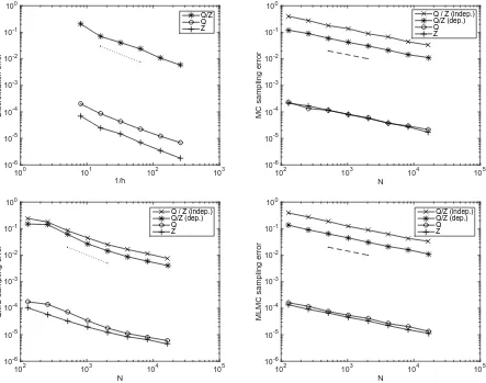
Figure 1: Convergence w.r.t. h of the discretisation errors _|Qh/Zh−Q2h/Z2h|, |Qh−Q2h| and

|Zh−Z2h|(top left), as well as convergence w.r.t. N of the sampling errorsE[(Qbh/Zbh−Qh/Zh)2]1/2,

E_[(Qb_h−Qh)2_]1/2 _andE_[(Zb_h−Zh)2_]1/2 _{for MC (top right), QMC (bottom left) and MLMC (bottom}

right), respectively. The dotted and dashed reference slopes are ₋1 and ₋1/2, respectively.

For the QMC estimators, we choose a lattice rule with product weight parameters γj = 1/j2

and one random shift. The generating vector for the rule used is available from Frances Kuo’s web-site (http://web.maths.unsw.edu.au/_∼fkuo/) as ”lattice-39102-1024-1048576.3600”. We point out here that this generating vector is a standard, off the shelf generating vector, rather than a generating vector specifically constructed for the weights implicitly defined in Assumption A4 and Lemma 4.1. In practice we found this generating vector to work well, even though the convergence rates in Lemma 4.1 were not proven for this particular choice.

6.1 Mean Square Error

Accuracy ǫ

10-2 10-1 100

Computational cost

103 104 105 106 107 108 109 1010

MC (dep.) QMC (dep.) MLMC (dep.)

ǫ-4 ǫ-3 ǫ-2

Accuracy ǫ

10-2 10-1 100

Computational cost

103 104 105 106 107 108 109 1010

MC (indep.) QMC (indep.) MLMC (indep.)

ǫ-4 ǫ-3 ǫ-2

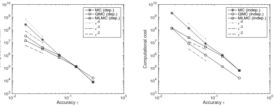
Figure 2: Computational cost of ratio estimators Qbh/Zbh to achieve a RMSE e(Qbh/Zbh) of ε, using

the same random samples in Qbh and in Zbh (left) and using different random samples inQbh and in

b

Zh (right), respectively.

Figure 1 shows the discretisation error and the sampling errors of the different estimators. The top left plot shows the discretisation error_|Qh/Zh−Q2h/Z2h|, as well as the individual discretisation

errors|Qh−Q2h|and|Zh−Z2h|. We see these errors decay linearly inh, as predicted by Theorem 3.3.

The other three plots show the sampling errorE_[(Qb_h/Zb_h−Qh/Zh)2_]1/2_{, as well as the individual}

sampling errorsE_[(Qb_h−Qh)2_]1/2 _andE_[(Zb_h−Zh)2_]1/2_{, for MC (top right), QMC (bottom left) and}

MLMC (bottom right). The mesh sizeh is fixed at h= 1/16, and the “exact” expected values Qh

and Zh are estimated with MLMC with a very large number of samples. For MC and QMC, N

on the horizontal axis represents the number of samples. For MLMC, N represents the equivalent number of solves on the finest grid h = 1/16 that would lead to the same cost as the MLMC estimator. This means that for a givenN, the cost of all three estimators is the same. The number of samples Nℓ in the MLMC estimator was chosen proportional to h−_ℓ(4s+γ)/2 ≈h−_ℓ2, as suggested

by the optimisation in [25, 6], assuming s≈1/2 and γ ≈2. We show results for ratio estimators with the same random samples used in Qbh and Zbh, referred to as dependent estimators, as well

as ratio estimators with different random samples used in Qbh and Zbh, referred to as independent

estimators. For MC and MLMC, we observe a convergence rate ofN−1/2_{. For QMC, we observe a}

convergence rate which is significantly faster than order N−1/2 and almost orderN−1.

Figure 2 compares the computational costs of the different estimators to achieve an RMSE ofε. The computational cost of the estimators was computed asN h−2 _{for the MC and QMC estimators,}

and as N0h−02 +

PL

ℓ=1Nℓ(h−ℓ2 +hℓ−−21) for the MLMC estimator. The bias |Qh/Zh −Q/Z| was

estimated from the values of_|Qh/Zh−Q2h/Z2h|shown in Figure 1. As predicted by Theorem 5.2

withγ _≈2 ands_≈1/2, the cost of the MC estimator grows with aboutε−4_{, the cost of the QMC}

estimator grows with aboutε−3, and the cost of the MLMC estimator grows with aboutε−2.

6.2 Dependency on m _and σ2

η

σ η

2

10-3 10-2 10-1 100

Sampling error

10-2 10-1 100 101

MC (dep.) QMC (dep.) MLMC (dep.)

m

100 101 102 103

Sampling error

10-2 10-1 100 101

MC (dep.) QMC (dep.) MLMC (dep.)

Figure 3: Sampling errors E_[(Qb_h/Zb_h−Qh/Zh)2_]1/2 _{as a function of noise level σ}2_{η (left) and as a}

function of number of observationsm (right), respectively.

µy to concentrate on a small region of the parameter space. The ratio estimators sample from the prior distribution and do not make use of this fact. We expect the sampling errors to grow with increasing m and decreasing σ2

η. To ameliorate this problem, one can under certain assumptions

rescale the parameter space before applying the ratio estimators, see e.g. [42] for details.

Figure 3 shows the sampling error of ratio estimators based on using the same samples in Qbh

and Zbh. We observe a mild growth of the sampling errors both with increasing m and decreasing

σ_η2, but the growth is not dramatic and all estimators appear to be robust over a large range of practically interesting values. The fact that the sampling error for MLMC based estimators grows more quickly than for MC and QMC based estimators, is at least partly caused by the fact that V_{[ψh0] and} V_{[ψh1 −ψh0] become of the same size for small ση}2 _{or large m, making the choice}

Nℓ =Ch−_ℓ2less and less optimal. Experiments with estimators based on using independent samples

inQbh andZbh also showed growth of sampling errors for small σ2η and large m, in fact much faster

than in the case of dependent estimators.

7

Conclusions and further work

uncertainty quantification.

It would be interesting to compare the performance of the ratio estimators considered in this work to Markov chain Monte Carlo (MCMC) and multilevel Markov chain Monte Carlo (MLM-CMC) methods [32, 18]. Especially in the case of small noise levelσ2_ηor large number of observations m, MCMC based approaches might explore the posterior distribution more efficiently. In terms of the ε-cost of estimators, the analysis and simulations in [18] show that the computational cost of a standard MCMC estimator grows at the same rate as a ratio estimator based on MC, and the cost of an MLMCMC estimator will grow at the same rate as a ratio estimator based on MLMC. The constants appearing in these estimates, for MCMC based approaches, depend on quantities like the acceptance rate, autocorrelation and possibly the dimension of the parameter space. For the high dimensional problems considered in this work, these constants might be very large.

A

Proof of Assumption A4 for

θ

_{for linear and scalar}

_H

Letm= 1, letH be a linear functional onV =H₀1(D) and letk∗_min:= min_x∈Dk∗(x)>0 and thus kmin(ξJ) ≥ k∗min > 0, for all ξJ ∈ RJ. Let us assume without loss of generality that y = 0 and

σ2

η = 1, and for simplicity letξ=ξJ ∈RJ. Then,θ(ph(·;ξ) =g(h(ξ)) withg(ζ) := exp(−ζ2/2) ≤1

andh(ξ) :=_H(ph(·;ξ)). To simplify the presentation, we writegn:=

dng

dζn(h(ξ)) andhµ:=

∂|µ|_h

∂ξµ (ξ) whereµis a multi-index in {0,1}J.

Let C be a generic constant independent of J, ν and ξ. First note that due to (3.3) and the

linearity ofH

|h(ξ)_{| ≤ kHkH}−1_(D)|ph|

H1 0(D)≤

kHkH−1_(D)kfk_H−1_(D)

k_min∗ =:κ∗.

Then, we have gn(ζ) = (−1)nHn(ζ)g(ζ) where Hn is the nth Hermite polynomial, and so

|gn(h(ξ))| ≤Cmax{1,|h(ξ)|n}g(h(ξ))≤Cmax{1, κn∗}. (A.1)

Moreover, it was shown in [26, Theorem 16] that, for linear H,

|hµ(ξ)| ≤κ∗

|µ|!

(ln 2)|µ|

J

Y

j=1

bµj

j . (A.2)

Now, Faa di Bruno’s formula for the special case whereν ∈ {0,1}J and whereh(ξ) is scalar (cf.

[10, Corollary 2.10]) states that

θν =

|ν|

X

r=1

gr

X

P(r,ν)

r

Y

i=1

h_µ(i)

where

P(r,ν) :=

(

µ(1), . . . ,µ(r) :0≺µ(1)≺. . .≺µ(r) and

r

X

i=1

µ(i)=ν

and_≺indicates some unique linear ordering of multi-indices (see [10, p. 505] for an example). And so, using (A.1) and (A.2), we get

|θν| ≤C

|ν|

X

r=1

max_{1, κr_∗} X

P(r,ν)

r

Y

i=1



κ∗ |

µ(i)|!

(ln 2)|µ(i)|

J Y j=1 bµ (i) j j   ≤C

max{κ∗, κ2∗}

ln 2

|ν|

 

|ν|

X

r=1

X

P(r,ν)

r

Y

i=1

|µ(i)|!

 

| {z }

=:ρν

J

Y

j=1

bνj

j

since all elements of P(r,ν) satisfyPr_i=1µ(i) =ν and Pr_i=1|µ(i)|=|ν|. It remains to bound ρν. We give a simple but fairly crude bound.

First note that, for each element (µ(1), . . . ,µ(r))∈P(r,ν), the moduli|µ(i)|,i= 1, . . . , r, form

a partition ofn:=|ν|. Hence, instead of partitioning the summands in ρν into the subsetsP(r,ν), we can also sum over all possible partitions k1, . . . , kr ofn with 1≤r≤n. The partition function

p(n) is the number of possible partitions of n. It is bounded by exp(πp2n/3) [13]. For each partition k1, . . . , kr of n, the number of possible elements inP(r,ν) that satisfy |µ_i|= ki can be

bounded by

n k1

n−k1

k2

n−P2i=1ki

k3

!

. . . n−

Pr−1

i=1 ki

kr

!

= n!

k1!k2!. . . kr!

Elements of P(r,ν) where |µ_i| = |µ_j|, for some i 6= j, are counted twice in this bound. Since

Qr

i=1|µ(i)|! =k1!k2!. . . kr!, we finally get the bound

ρν ≤p |ν|

|ν|!≤exp π

r

2_|ν|

3

!

|ν|!.

Hence, there exists a constantcp >1 such that Assumption A4 holds withc1 :=cpmax{κ∗, κ2∗}/ln 2.

References

[1] S. Agapiou, O. Papaspiliopoulos, D. Sanz-Alonso, and A. M. Stuart, Importance sampling: computational complexity and intrinsic dimension. Available as arXiv preprint arXiv:1511.06196. [2] A. Barth, Ch. Schwab, and N. Zollinger,Multilevel Monte Carlo finite element method for elliptic

PDE’s with stochastic coefficients, Numer. Math., 119 (2011), pp. 123–161.

[3] R.C. Ceary, The frequency distribution of the quotient of two normal variables, J. Roy. Statist. Soc, 93 (1930), pp. 442–446.

[4] J. Charrier,Strong and weak error estimates for the solutions of elliptic partial differential equations with random coefficients, SIAM J. Numer. Anal, 50 (2012), pp. 216–246.

[5] J. Charrier, R. Scheichl, and A. L. Teckentrup,Finite element error analysis of elliptic PDEs with random coefficients and its application to multilevel Monte Carlo methods, SIAM J. Numer. Anal., 51 (2013), pp. 322–352.

[7] A. Cohen, R. DeVore, and Ch. Schwab,Convergence rates of best N-term Galerkin approximations for a class of elliptic SPDEs, Found. Comput. Math., 10 (2010), pp. 615–646.

[8] N. Collier, A.-L. Haji-Ali, F. Nobile, E. von Schwerin, and R. Tempone, A continuation multilevel Monte Carlo algorithm, BIT Numerical Mathematics, 55 (2014), pp. 399–432.

[9] P. R. Conrad, Y. M. Marzouk, N. S. Pillai, and A. Smith, Accelerating asymptotically exact MCMC for computationally intensive models via local approximations, J. Amer. Statist. Assoc., (2015).

[10] G. M. Constantine and T. H. Savits, A multivariate Fa`a di Bruno formula with applications, Trans. Amer. Math. Soc., 248 (1996), pp. 503–520.

[11] S. L. Cotter, G. O.Roberts, A. M. Stuart, and D. White, MCMC methods for functions: modifying old algorithms to make them faster, Stat. Sci., 28 (2013), pp. 424–446.

[12] M. Dashti and A.M.Stuart,The Bayesian approach to inverse problems, in Handbook of Uncertainty Quantification, R. Ghanem, D. Higdon, and H. Owhadi, eds., Springer, 2015.

[13] W. de Azevedo Pribitkin, Simple upper bounds for partition functions, Ramanujan J., 18 (2009), pp. 113–119.

[14] J. Dick, R.N. Gantner, Q.T. Le Gia, and Ch. Schwab,Higher order quasi-Monte Carlo integra-tion for Bayesian estimaintegra-tion, arXiv preprint arXiv:1602.07363, (2016).

[15] J. Dick, R. N. Gantner, Q. T. Le Gia, and Ch. Schwab, Multilevel higher order quasi-Monte Carlo Bayesian estimation, Tech. Report 2016-34, Seminar for Applied Mathematics, ETH Z¨urich, Switzerland, 2016.

[16] J. Dick, F.Y. Kuo, and I.H. Sloan, High-dimensional integration: The quasi-Monte Carlo way, vol. 22 of Acta Num., Cambridge University Press, 2013, pp. 133–288.

[17] C. R. Dietrich and G. N. Newsam, Fast and exact simulation of stationary Gaussian processes through circulant embedding of the covariance matrix, SIAM J. Sci. Comput., 18 (1997), pp. 1088–1107.

[18] T.J. Dodwell, C. Ketelsen, R. Scheichl, and A.L. Teckentrup, A hierarchical multilevel Markov chain Monte Carlo algorithm with applications to uncertainty quantification in subsurface flow, SIAM/ASA J. Uncertainty Quantification, 3 (2015), pp. 1075–1108.

[19] P. Doukhan and G. Lang,Evaluation for moments of a ratio with application to regression estima-tion, Bernoulli, 15 (2009), pp. 1259–1286.

[20] D. Elfverson, F. Hellman, and A. M˚alqvist, A multilevel Monte Carlo method for computing failure probabilities, SIAM/ASA Journal on Uncertainty Quantification, 4 (2016), pp. 312–330.

[21] E.C. Fieller, The distribution of the index in a normal bivariate population, Biometrika, (1932), pp. 428–440.

[22] C. Galeone and A. Pollastri,Confidence intervals for the ratio of two means using the distribution of the quotient of two normals, Statistics in Transition, 13 (2012), pp. 451–472.

[23] R. N. Gantner and M. D. Peters,Higher order quasi-Monte Carlo for Bayesian shape inversion, Tech. Report 2016-42, Seminar for Applied Mathematics, ETH Z¨urich, Switzerland, 2016.

[24] R. G. Ghanem and P. D. Spanos, Stochastic finite elements: a spectral approach, Springer, New York, 1991.

[25] M. B. Giles,Multilevel Monte Carlo path simulation, Oper. Res., 256 (2008), pp. 981–986.