Microwave power amplifier design using stack topology

(1)

M

ICROW

WAVE

U

SIN

E

P

OW

NG STA

Gü

TNO

Ir. M

UT

Pro

11

WER

A

ACK T

By

ürhan Vu

O

Superv

Marc van

Supervis

f.dr.ir. Fr

1-08-2011

A

MPLI

TOPOL

ural

visor:

Heijning

sor:

rank van V

FIER

D

LOGY

gen

Vliet

D

ESIG

(2)

(3)

3

1. INTRODUCTION ... 5

1.1 Goal of design ... 6

1.2 active device technologies in power amplifiers for radar applications ... 6

1.3 Organization of Thesis ... 9

2. Overview of power amplifiers ... 10

2.1 Power amplifiers working as a current source ... 10

2.1.1. CLASS A Amplifier ... 11

2.1.2. CLASS B Amplifier ... 12

2.1.3 Class C power amplifiers ... 13

2.1.4 Class AB power amplifiers ... 13

2.2 switch mode power amplifiers ... 13

2.2.1 class F Power amplifiers ... 14

2.2.2 class E Power amplifiers... 14

2.3 Disadvantages of switch mode PAs ... 20

3. cascode architecture ... 20

3.1 POSSIBLE CASCODE CONFIGURATIONS ... 21

3.2 why an additional capacitor must be added on the gate of the second transistor? ... 22

4. performance analysis of stacked mmic power amplifier in GaAstechnology using ads ... 28

4.1 Linear pa design to verify the stacked structure concept for s band system ... 28

4.1.1 Linear single gate design ... 28

4.1.1 stacked Configuration Biased in Class AB-mode ... 33

4.1.2 performance of designed unmatched class ab pa ... 36

4.2 switch mode design as an alternative approach to linear design in order to improve the efficiency ... 37

4.2.1 Single stage class –E @3.2 GHz ... 38

4.2.2 stacked switch mode design ... 41

4.2.3 performance summary of designed switch mode pa ... 44

4.3 impedance matching network design for linear power amplifier ... 45

4.3.1 Input/output matching circuit design for common source stage PA ... 46

5. circuit schematic of the designed cascode ‘linear’ pa with non‐ideal components ... 59

5.1 performance of the pa with non ideal components ... 62

(4)

4

Figure 5.7: The layout of the whole circuit ... 65

6 conclusions and recommendations ... 65

(5)

5

1.INTRODUCTION

Power amplifiers for radar applications require a relatively wide bandwidth (for example from 8.0 -12 GHz) and need to deliver as much output power as possible. Therefore these

amplifiers are designed to the limit of what is offered by the used processing technology. The main limit is the voltage breakdown of the transistors. For typical GaAs processing

technologies this gate-drain voltage breakdown limit is around 16 to 20 V, and typical drain bias voltage is around 8 V.

In standard class- AB amplifier designs the voltage swing at the output of the transistors is around 2 times the drain bias. Therefore the maximum drain bias is around half of the breakdown voltage limit (with some correction for the knee region and extra margin for reliability). This maximum drain bias (together with the maximum current) defines the maximum output power.

Given a fixed technology and transistor size the current cannot be increased. The only way to increase the output power any further is to increase the voltage swing. One way of doing this is to use a cascode transistor: the combination of a common gate transistor (either as two separate transistors or as one dual gate transistor). This approach is often used in low voltage CMOS technology, where the bias voltage is limited to only 1.1 V

This approach is also often used in very high frequency designs, where the gain offered by the cascode is higher than that of a single common source transistor. A cascode configuration also offers more bandwidth and is therefore often applied in very wide band distributed amplifiers.

In this thesis following study questions will be investigated.

 For what applications are cascodes currently used, and why? (What is the theory

behind cascodes?)

 Can cascode transistors be used to increase the output power of microwave power

amplifiers in the range of S- band (2 to 4 GHz)?

 Are cascode devices useful for other operating classes, such as Class-E, Class-F, etc.,

where higher drain voltage peaks can occur?

 Can a microwave power amplifier with cascodes offer more bandwidth (while

delivering at least the same output power and efficiency) than standard power amplifiers (using only common source devices)?

 What specific modeling is required for cascodes (especially for the common-gate

device)?

 What implementation of cascodes is most useful: 2 separate devices (common source

+ common gate, or a dual-gate device)?

 Demonstrate the use of cascodes by designing a microwave integrated power amplifier

(6)

6

To be able to answer the above described research questions, literature information will be provided together with simulation results in ADS. Following design goals will be achieved with employing aforementioned cascode concept at S band.

1.1

G

OAL OF DESIGN

Increase the output power of microwave power amplifiers and/or increase the maximum Power Added Efficiency,

For:

• Microwave (>2 GHz) integrated power amplifiers (MMICs)

• In GaAs technology ( 0.5um pHEMT, TNO model)

Target specifications

For S-band Bandwidth: 2.9 – 3.5 GHz

We start with background information about the power amplifiers for radars.

1.2

ACTIVE DEVICE TECHNOLOGIES IN POWER AMPLIFIERS FOR RADAR APPLICATIONS

There are several active device technologies that are mostly used in radar applications. Most important technologies that are used are based on GaAs, LDMOS and GaN which is the new generation amplifier technology.

LDMOS-based Amplifiers

LDMOS is an enhanced MOSFET structure especially suited for high power applications. It is used from point-to-multipoint communications to Radar. The most pervasive application is in cell phone base-stations. [5]

These technologies are best known to operate with supply voltages of 28V with recent improvements allowing 50V operation

(7)

GaAs-b In today provide operatin Higher p applicat indispen sense of GaN- b As men higher t higher o GaN HEM The wi supply v amplifie amplifie are both Figure 1 based Amp

y radar syste high-effici ng from sup

power radar tions GaAs nsable for th f bandgap a

based Amp

ntioned befo than the GaA

output. Com

MTs have sm

de bandgap voltage up t ers for radar ers. The maj h costly and

1.1 summar

Figu

lifiers:

ems GaAs i ency and th pply voltage

r applicatio device has hose applica and power d

plifiers

ore GaN tech As devices

mpared to sil maller paras

p character o to 1000 volt r application ajority of Ga d limited in s

ries the abov

re 1.1: Radar

is the one of hat operate i es ranging fr

ns require d power dens ations. GaN density whic

hnology has [32]. This h

icon LDMOS sitic capacita

of GaN resu t. It is the be ns today. Bu aN HEMTs

size.

ve mentione

Amplifier Te

f the most u in microwav rom 5V to 2

devices with sity limitatio N has better

ch omit thes

s a very hig higher densi

S FETs and G ances. [28]

ults in a high est candidat ut the cost i are produc

ed PA techn

echnology Ada

used technol ve and milli 28V. [28]

h higher pow on. Therefo

physical pr se limitation

gh power de ity results in

GaAs MESFE

her breakdo te for the ne is the main ed on silico

nologies

aptation Proje

logy. GaAs imeter frequ

wer density re power co operties tha ns of GaAs.

nsity which n a smaller t

ETs of simila

own voltage ext-generati drawback o on carbide su

ection [4]

-based amp uency range

y. For these ombining is an GaAs in

h is about te transistor d

ar output po

e and allow ion power of these type

(8)

In semicon

T

Because technolo

Fig

frequen

n de table 1 nductor mat

Table 1.1: S

e of the goo ogies at hig

gure1.2: Po cy.[33]

.1 we see th terials for R

Semiconduc

od power pe gh frequenci

ower perfor

he comparis RF and micro

ctor materia

erformance o ies we will d

rmance of H

son of mater owave appl

als for RF an

of GaAs PH design our P

EMTs, MESF

rial properti lications.

nd microwa

HEMT comp PAs with us

FETs and HB

ies of GaN w

ave applicati

pared to the sing this as

BTs as a fun

with other

tions [29]

e other devi active devic

nction of

8

(9)

9

1.3

O

RGANIZATION OF

T

HESIS

The goal of this thesis is, to increase the output power and/or increase the maximum power added efficiency (PAE) of a microwave power amplifier in GaAs technology.

Introduction and power amplifiers for radar applications are described above in chapter 1

The thesis is organized as follows:

Chapter 2 presents the specification for the high power amplifier (HPA) design and selected operating HPA operating class.

Chapter 3 deals with explanation of the functioning, use and advantages of cascode structure.

Chapter 4 discusses the design issues. Unit cell (cascode) performance and bias point

selection, output matching, input matching, total performance of the whole circuit and layout is presented in this chapter.

Chapter 5 represents the designed PA with design kit components and the layout

(10)

10

2.

O

VERVIEW OF POWER AMPLIFIERS

Power amplifiers can be categorized into two major groups [5]: Linear PAs and Nonlinear PAs. Linear PAs are able to generate output power proportional to the input power with a negligible amount of harmonic power generated. On the contrary, non-linear Pas operate near the cut-off region with a significant amount of harmonics generated besides the fundamental signal. The input and output power are no longer proportionally related.

Furthermore, amplifiers can also be classified into 2 categories: biasing class and switching class. In biasing class, amplifiers such as Class A,B, AB and C amplifiers are classified based

on their quiescent point (bias point) or output Current Conduction Angle (CCA) θ. θ is

defined as the fraction of RF input drive signal where non-zero current is flowing through the device [5].

In this thesis we will investigate the benefits of stacked topology with circuits both in linear and non linear characteristics. This will provide us a good comparison opportunity whether we can make use of power efficiency enhancement using switch mode power amplifiers for MMIC power amplifiers at high frequencies. In this way we will try to increase the output power about 2 times more than a common source stage and at the same time keeping a relative high PAE.

For linear PA design case the circuit will be biased in class AB mode according to reason that will be explained in the coming section. In non linear case we will use a class E switch mode power amplifier because of the reasons which are also be explained in the coming sections.

2.1

P

OWER AMPLIFIERS WORKING AS A CURRENT SOURCE

In PAs working as a current source, different bias points result in different conduction angles, and therefore different classes of operation with each having own pros and cons. Here we will briefly describe each class of operation. The detailed analysis and derivation of the linear power amplifiers are fully discussed elsewhere (see e.g. [7], [8])

Efficiency for linear PA can be given in general form as follows [9].

For the voltage and current we have (see fig 4.1),

cos

in b in

v  v V  t, (2.1)

cos q

i I  I ; For -θ<ωt<θ; otherwise i=0, (2.2)

in which Vb is the bias voltage, Iq is the quiescent current, θ is the half of the conduction

angle, and Vin and I are amplitude of the input voltage and the output current respectively

Since θ is the half of the conduction angle, it can be determined at the moment when current

(11)

11

cos 0 cos q (cos cos ) 0

q

I

I I i I t t

I

   

          (2.3)

In order to determine the efficiency for each class of operation, first the DC component of the current and the fundamental component of it should be calculated using (2.4) and (2.5),

0

1

(cos cos ) (sin cos ) 2

I

I I t d t



     

 _ 





   (2.4)

1

(cos cos ) cos ( sin cos ) 2

I

I I t td t



      

 _ 





   (2.5)

Knowing that the efficiency is the ratio of power at the fundamental to the power at DC, and assuming an ideal condition of zero saturation voltage (voltage peak factor (Vin/Vcc) is equal to 1, in which Vcc is the DC supply voltage), we have,

1 1

0 0

2 0 0

1 1 ( sin cos ) 2 2 (sin cos )

2

P I

V P

R

  



  

     

 

(2.6)

Depending on the conduction angle, efficiency and linearity of each class is determined. More details on different classes of operation of this category will be provided in the following sections.

2.1.1.

CLASS

A

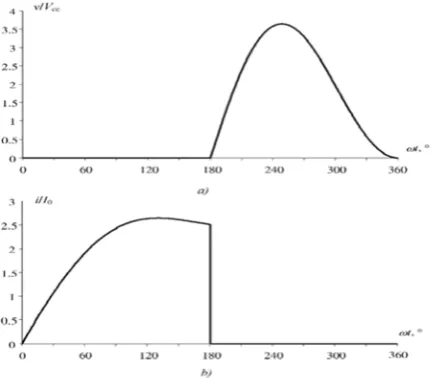
MPLIFIER

A Class A amplifier is a linear amplifier, which has conduction angle of 360°. The 360° conduction angle means that the transistor in this class is turned on and conducts over the entire sinusoidal cycle. Most of the small-signal amplifiers are designed in this class because of its simplicity and the best linearity among all classes of amplifiers. Because of the 360° conduction angle of Class A, these amplifiers have the lowest efficiency and are only suitable for low-power applications. The transfer characteristic of a Class A amplifier and its

corresponding voltage and current waveforms are shown in Fig.2.1

The class A amplifier is cheap, because it only requires a single active device. It is biased in the active linear region and amplifies the signal over the entire input cycle. Fig. 2.1 shows how a class A amplifier operates. Its performance is good in terms of linearity (it contains no harmonics at the output), but undesirable in terms of efficiency. In other words, it is very inefficient because it is always conducting even when there is no input signal. According to

(12)

2.1.2.C

Unlike c operatio dissipat not pure linear. U obtainab

Figu

CLASSBAM

class A, a c on is shown tion, but on ely sinusoid Using (2.6) ble for a cla

ure 2.1: Volt

MPLIFIER

lass B ampl n in Fig. 2.2. the other ha dal anymore

with θ=90°

ass B power

Figu

tage and curr

lifier amplif . Turning of and, increas e. Therefore (half the cy r amplifier.

ure 2.2: Cla

rent waveform

fies only ha ff the ampli ses the harm e, class B is

ycle) shows

ass B operati

ms in

Class-alf of the cyc ifier for half monic conten

more effici s that a max

on

A operation.

cle of the in f of the cycl nt of the ou ient than cla ximum effici .

nput signal. le reduces p utput signal

ass A but le iency of 78

12

Its power

(13)

13 2.1.3CLASSCPOWERAMPLIFIERS

A class C amplifier conducts even less than half of the cycle of the input signal (θ is less than

90°), which makes it more efficient than class B. But it should be noted that the advantage of high efficiency comes with the disadvantage of high distortion at the output.

2.1.4CLASSABPOWERAMPLIFIERS

The class AB amplifier is a classical compromise, which has higher efficiency than class A, but inevitably increased nonlinearity [8]. In other words, the class AB amplifier is biased somewhere between class A and class B (which means less than full cycle but more than half a cycle conduction). Therefore, the ideal efficiency will be between 50% and 78.5% (feasible PAE 40-50%), and the linearity will be better than a class B, but worse than a class A

amplifier.

Since in our design, efficiency and output power is more important than the linearity; our choice for biasing will be in class AB mode.

Following section will analyzes the switch mode power amplifiers. Among different class of switch mode power amplifiers class E type power amplifiers gain more attention since class E power amplifiers can better tolerate real circuit variation[10] and also it has a relative simple configuration compared to the other switching modes PAs. Therefore our attention will be focused mainly on this class of amplifiers.

2.2

SWITCH MODE POWER AMPLIFIERS

In this category, power amplifiers are designed so that the transistor acts as an RF switch, rather than as a voltage-controlled current source. In other words, the output networks provide non-overlapping waveforms. Furthermore, efficiency of this category is improved, because of operation in the saturation region at the cost of more complex load networks (which means at lower powers, switching mode power amplifiers will have poor efficiency). On the other hand, linearity is sacrificed due to operation in a strongly nonlinear region, which results in nonlinear voltage and current waveforms.

(14)

2.2.1CL Class F overlap termina Fig.2.3 As show wave sh harmon harmon 2.2.2CL As men gain mo variatio

In the C the curr voltages power a amplifie [11]. There ar shunt ca wave tra

LASSFPOW

power amp between cu ations. Ideal

Figu

wn in Fig. 2 hape. The cu

ics. It result ics. Theoret

LASSEPOW

ntioned in 2 ore attention

n[10].

Class E pow rent and vol s do not ove amplifier eff er by an app

re different apacitance,

ansmission

WERAMPLIF

plifiers are a urrent and v current and

ure 2.3 Ideal

2.3, the curre urrent conta

ts in non ov tically, an id

WERAMPLIF

2.1.4 , betwe n since class

wer amplifier tage wavefo erlap simult fficiency. Su propriate ch

class E pow even harmo line. Here w

FIERS

analyzed in voltage is do d voltage wa

current and

ent wavefor ains the even verlapping h

deal efficien

FIERS

een the swit s E power a

r, the transis orms provid taneously, to uch an opera hoice of the

wer amplifie onic Class E we will shor

the frequen one in the fr aveforms of

voltage wav

rm is half-si n harmonic harmonics a ncy of 100%

tching mode amplifiers ca

stor operate de a conditio

o minimize ation mode

values of th

ers configur E, parallel-c

rtly deal wi

ncy domain. requency do f a class F p

veforms of cl

inusoidal an s, while vol and reductio % is predict

e amplifiers an better to

es as an on-o on where th the power

can be real he reactive e

rations avai circuit Class ith these con

In other wo omain using power ampli

ass F power

nd the volta ltage consis on of the pow

ted.

s class E typ olerate real c

off switch a he high curr

dissipation ized for the elements in

ilable namel s E, and Cla

nfigurations

ords, cance g harmonic lifier are sho

amplifier

age has a squ sts of odd

wer loss du

pe power am circuit

and the shap rent and hig

and maxim e tuned pow n its load net

ly; Class E ass E with q s and in the

(15)

followin wave tra

2.2.2.1

The bas where th

L, a seri

transisto fundam as their differen 2.2.2.2 The sec than ide Class E resonan output v resonan tuned on 2n   The loa capacita collecto ng sections, ansmission

1ClassEw

sic circuit of he load netw ies fundame or is connec mental freque electrical b ntial equatio

Figu

2Evenhar

cond-order C eal RF chok

, the DC fee nce conditio

voltage acro nce conditio

n any even

1

LC Wher

d network o ance Cxis n

or voltage (a

, we will als line in orde

withshunt

f a class E p work consis entally tune cted to the s ency. Such behavior in t ons. (See for

ure 2.4 Basic

rmonicCla

Class E load ke with infin ed inductan n and it is a oss the load n means tha harmonic c

re n =1, 2, 3,

of the even h needed to co

a) and curre

so provide t er to compar

tcapacitan

power ampl sts of a capa

d L C₀ ₀ circ

supply volta a simplified time domain r more detai

c circuits of C

assE

d network im nite reactanc nce is restric

assumed tha have a pha at the parall omponent:

, …

harmonic C ompensate th

nt (b) wave

the ADS sim are the perfo

nce

ifier with a acitance C s

cuit and a lo age by RF c d load netwo

n can be ana ils [12]).

Class-E pow

mplies the f ce at any ha cted to value at the fundam

se differenc lel inductan

Class E is sh he required eforms for id

mulation res ormance of t

shunt capac shunting the oad resistanc hoke having ork represen alytically de er amplifier finite value armonic com

es that satis mental volt ce of π/2. G

nce L and sh

hown in Figu phase shift dealized op

sults of Clas this SMPA

citance is sh e transistor,

ce R. The co

g high react nts a first-or escribed by

with shunt c

of DC feed mponents. F

fy an even h age across t enerally, ev hunt capacita

(2

ure 2.5 whe . In Figure 2 timum even

ss E with qu with the lin

hown in Fig a series ind ollector of t tance at the rder Class E y the first-or

capacitance. [

d inductance For even har harmonic the switch a ven harmoni ance C can

2.7)

(16)

mode ar similar t the curr configu DC curr driving current

F

re plotted. A to the collec rent wavefor uration, the c rent, at the e signal it is i is smoothly

Figure 2.5 E

Figu

Although th ctor voltage rm is substa collector cu end of the c impossible y reducing t

Equivalent ci

ure 2.6 Norm

o

e collector v e waveform antially diff urrent reache

conduction i to provide t o zero. [12]

rcuit of the e

malized collec optimum eve

voltage wav m of Class E

ferent. So, fo es its peak v interval. Co the maximu ]

even-harmon

ctor voltage en harmonic

veform of e with shunt for the even value, which onsequently um collector

nic Class-E p

(a) and curre Class E. [12

ven harmon capacitance harmonic C h is four tim , in the case r current wh

power amplif

ent (b) wavef ]

nic Class E e, the behav Class E mes greater

e of the sinu hen the inpu

fier. [9]

forms for ide

16

is very vior of

than the usoidal

ut base

(17)

2.2.2.3 The loa circuit i voltage paramet parallel-Figure 2 optimum resistan

QLassu

F

3Parallel‐

d network o is tuned to th

and current ters, a paral -circuit Cla 2.8, the norm m condition nce R, parall

umption for

R

Figure 2.7: E

Fig

circuitCla

of a parallel he fundame t waveform llel inductan

ss E mode, malized col ns are shown

lel inductan the series L

2 1.365 cc out V P Equivalent c

gure 2.8: No

(b) For a

assE

l-circuit Cla ental frequen

s is provide nce L, a shu

no addition llector volta n. For the p ce L and pa

0 0

L C circuit

L

ircuit of the

ormalized co an idealized

ass E amplif ncy and the ed by the pr unt capacitan

nal series ph age (a) and c arallel-circu arallel capac t [12]: 0.732R  parallel-circu ollector volt optimum pa

fier is shown e required ph oper choice nce C and a

hase-shifting current (b) w uit Class E m citance C ca

C 

uit Class E p

tage (a), and arallel circu

n in Figure hase shift to e of the three a load resista g elements a waveforms mode, the o an be obtain

0.685

R



power amplif

d current wa uit Class E. [

2.7. The se o realize ide

e parallel ci ance R. In t

are required for idealize optimum loa ned, with the

[image:17.595.160.380.453.642.2]

(18)

2.2.2.4

The ide transmis

0 0

L C ci

current transmis

R with h

[image:18.595.146.403.441.517.2]

Class E even an the shun At even the freq conditio with a q conditio circuit. Figure 2 The the (see [9] simple l this case impedan even ha compon output m quarter-circuit c

4ClassEw

alized Class ssion line is ircuit is show

(b) wavefor ssion line ar

high QLassu

R

mode with nd odd harm nt capacitan n harmonics quency prop ons at odd h quarter wave ons typical f

[12]

2.9: Equivale

oretical resu for detail m load networ e, the shunt nce at the fu armonics. Th nent. Conseq matching cir -wave transm condition at withquart

s E load net s connected wn in Figur rms for an i re shown. T umption for 2 0.465 cc out V P

a quarter w monics. At o

nce as it is re , the optimu erties of a g harmonics an

e transmissi for both Cla

ent circuit of

ults obtaine mathematica

rk to realize t capacitanc undamental hen, an open quently, wh rcuit, the op mission line t the third-h

erwavetr

twork with a d between th

re 2.9. In Fi idealized op The series in r series L C₀

L wave transm dd harmoni equired for um impedan grounded qu nd short cir ion line to c ass E with a

f Class E pow

ed for Class al derivation e the optimu

e C and ser

and the qua n circuit con hen the idea

ptimum imp e can be pra armonic com

ransmissi

a shunt cap he series ind

igure 2.10, t ptimum Clas

nductance L

0

C circuit ca

1.349R



mission line ics, the optim

all harmoni nces are rea uarter wave rcuit conditi combine sim a shunt capa

wer amplifier

E mode wi n of these re um impedan ries inductan

arter wave t ndition is re al series L C₀

pedance con actically ful mponent. (S ionline acitance wh ductance and the normaliz ss E mode w

L, shunt cap

an be obtain

C 

shows diffe mum imped ics in Class alized using

transmissio ions at even multaneousl acitance and

r with quarte

ith a quarter esults) that nce conditio

nce L provid

transmission equired for

0

C circuit in

nditions for lly realized b

See figure 2

here a quart d fundamen zed collecto with a quart acitance C a

ned from

0.2725

R



erent impeda dances can b E with a sh a parallel L on line, with n harmonics

y the harmo d Class E wi

er wave trans

r wave trans it is enough ons even for de optimum n line realiz the third ha n figure 2.9

Class-E loa by simply p 2.10)

ter wave ntally tuned

or voltage (a ter wave and load res

(2.9)

dance proper be establish hunt capacit LC circuit. h its open c s, allow Cla onic impeda ith a paralle

smission line

smission lin h to use a ve r four harmo m inductive

zes the redu armonic is replaced ad network providing an 18 series a) and sistance rties at hed by tance. Thus, ircuit ss E ance el e [12]. ne show ery onics. In uction of

(19)

open-Figure 2 [9] The par equation harmon reactanc it is eno to provi the stan normall Thus wi simple c perform

2.10 Schema

rameters of ns that are g

ic compone ce of the pa ough to use ide the requ ndard load im

ly the case f

ith this type circuit. Bec mance with t

atic of quarter

the matchin given in 2.1 ent is used a

rallel third h the shunt ca uired impeda mpedance o for high-pow 1.34 0.27 0.46 L C R    

e of class E ause of this this type of

r-wave-line C

ng-circuit el 0. Here the

and Cb repre

harmonic ta

apacitance C

ance matchi

of R_L  50

wer or low-v

2 49 725 65 dd out R R V P  

PA, one can s reason we

switch mod

Class-E pow

lements can e parallel re esents the b ank circuit i

C2 composi

ing of the o

. In this ca

voltage pow

Q

C

L

C

n achieve a will investi de PA.

wer amplifier

n be calculat esonant L C₁

locking or b is inductive ng the L-typ ptimum Cla ase, it is assu wer amplifie 2 0 1 0 1 2 0 1 8 9 1 9 L L L L L R Q R Q C R Q R L C L         good harm igate our ca

with lumped

ted accordin

1 circuit tun

bypass capa at the funda pe low-pass ass-E load r umed thatR ers.

1 

monic termin scode PA st

d matching c

ng to the fol ned to the th acitor. Since damental fre

s matching resistance R

L

RR , whic

(2.10

nation with r tructure 19 circuit. llowing hird e the equency, circuit

R with

ch is

)

[image:19.595.151.410.74.230.2]

(20)

20

2.3

D

ISADVANTAGES OF SWITCH MODE

PA

S

It is also important to note that switch mode amplifiers are not suited for microwave application where broadband width is required since the design procedure of these class of operations is based on considering a single fundamental frequency, which makes it

narrowband and unsuitable for broadband power amplifiers. Another drawback of switch mode PAs is that although switch mode PAs achieves much higher efficiencies they generate strong nonlinearities.

A large output capacitance and switch on resistance (Ron) are also limiting factors at high

frequencies. At very high frequencies (at -wave range) this can cause deviation from the

ideal drain/collector voltage- current waveform for switch mode PAs which in turns result in an overlapping of both signal quantity. This will have then, of course, deleterious effect on the efficiency.

However there are some papers have been published with promising results at S band with switch mode PAs. In [6] PAE of greater than 70% over 3.0-3.7 GHz is obtained for 15.0 dBm input power drive, and a peak PAE of more than 90% is obtained at around 3.25 GHz when the amplifier is driven by only 12.0 dBm of input power. Over 10% bandwidth in S-Band, an inverse class-F amplifier exhibits [13] more than 60% drain efficiency and 10W output power. Also in [14] and [15] peak PAE performances close to 80% have been published for class-F and inverse class-F GaN power amplifiers operating at around 2GHz. We have to also stress out here that these designs are not all of them MMIC applications. A more general conclusion will be given after comparing the performance results of class AB PA with switch mode class E PA.

In the coming sections we will compare the performance of both, linear and switch mode PAs through simulation results. In this way we want to conclude that despite of those

aforementioned disadvantages of switch mode PAs, whether we can still achieve an acceptable relative broadband characteristic and enough output power and PAE for S band system with the aid of stacked- switch mode PA.

3.

CASCODE ARCHITECTURE

The cascode configuration is formed by a cascade of a common source (CS) stage driving a common gate (CG). (See figure 3.1) The cascode configuration is usually used for low-noise amplifier applications when a mixer is the next stage [B.Razavi et.al]. Then the load will be capacitive which will limit the frequency response of the LNA due to Miller effect. Also it is frequently used in wideband amplifiers because of high reverse isolation and high gain characteristic of the cascode configuration.

(21)

3.1

PO

There ar gate dev A dual-g cascode CS/CG vector n causes a The cas simpler The disa

OSSIBLE

C

re two type vices (as CS

Fi

gate device e pair, but oc

pair as it is network ana accuracy pr

code cell (d CS stage:  The effe  The but  Ano swin  The depe line  A du

effic  Dua

devi

advantages

ASCODE

C

s of cascode S+CG) and

igure 3.1 Sch

is electrica

ccupies less

a three por alyzer which

oblems [18]

dual gate an

output to in ct capacitan output imp the cascode other possib ngs at the ou

effective G endent on in arity perfor ual gate dev ciency could al gate devic

ice. [17, 18]

associated

CONFIGU

e arrangeme

a dual gate

hematic diag

ally equivale

s die area.

rt device and h needs a m

]

nd/or CS+CG

nput feedba nce is small pedance is h e cell is less ble advantag

utput before

Gds (output nput voltage

mance than vice has mu d be obtaine ce has highe

]

with dual g

URATIONS

ent possible device. (Se

gram of

dual-ent to a com [17]. Dual d only two-more comple

G combinat

ack capacita ler thereby a higher. Not o s sensitive to ge of the cas e FET break

conductanc e Vgs than t n single gate uch lower G

ed.

er maximum

gate device:

S

e one with a ee fig 3.1)

-gate FETs a

mmon-sourc -gate FET d port S-para ex modeling

tion) has som

ance is reduc allowing wi

only is the r o change in scode config kdown is re

ce) of the du the single g e device. Gds (higher R

m stable gai

a combinatio

and CS. /CG

ce (CS) / com differs in mo

meters are m g techniques me advanta ced; therefo ider bandwi reverse isola ds

r (drain s guration is h

ached.

ual gate dev gate device,

Rds), lower

n (MSG) th

on of two si

pair

mmon-gate odeling than measured u s which in tu

ages over th

ore, the Mill idths.

ation is very source resis

higher volta

vice is less resulting in

r loss hence

han single g

(22)

22

 Number of gates per device is twice of a single gate one, hence higher yield is

required during the processing, this practically becomes an issue

 A dual Gate device has higher knee voltage Vknee than the single gate one.

 Due to the complexity, it is difficult to get an accurate nonlinear model for the

dual gate device. [17,18]

Following argument explains the lower feedback of the cascode configuration. For better understanding of this argument, definition of Miller effect has to be given first. The Miller effect accounts for the increase in the equivalent input capacitance of an inverting voltage amplifier due to amplification of the capacitance between the input and output terminals. The additional input capacitance due the Miller effect is given by [2]

(1 )

m v gd

C  A C (3.1)

Loaded with the input impedance 1

m

g of the common gate circuit, the small signal gain, Av,

of the common source stage with transconductance g_m exhibits a low value of -1 since

m L

Av  g R .

According to Eq. (3.1) we get

(1 ) 2

m v gd gd

C  A C  C (3.2)

In comparison to the common source circuit this result in a much smaller Miller capacitance than the one for the common source circuit. Consequently, the low pass characteristic

associated with the input capacitance is less pronounced yielding higher cutoff frequencies for the voltage, current and power gain. [3] .The nearly unilateral nature of cascode cell helps improving the stability as well.

As it can be seen from the figure 3.1 an additional capacitor is added on the gate of the 2nd

transistor. Next section will highlight the reason of this configuration.

3.2

WHY AN ADDITIONAL CAPACITOR MUST BE ADDED ON THE GATE OF THE SECOND TRANSISTOR

?

The capacitor at the gate of the common gate transistor enables to equalize the output

(23)

Figu

On the o transisto transisto cell by c

Howeve stability the drain To get m should b the both

The out source d

ure 3.2: Schem

other hand, or makes it or. It enable considering

er during th y problems. n. Therefor more output be the same h transistor i

tput power o device Pout

Pou

In op

matic of balan

the addition possible to es to equaliz g that Ca2 m

he simulation This is due e in our des t power, the e. Thus both is achieved

of the balan tCS is derive



1 . [ 2

cas

ut  

ptimum pow

V

nced cascode c

n of a Ca2 c obtain twic ze the outpu meets the fol

2

n it is obser e to the fact sign Ca2 is r

voltage sw h have nearl by means o

nced cascode ed as follow



Vds1Vds2

wer case:

1

2 .

2 dd

Vg  V

cell with the a

capacitor be ce the outpu ut impedanc llowing requ

2 ∗

rved that ad that adding removed. wing across t

ly the same of the gate c

e configura ws in [16] (S



2 1 .( . .( 2 gm V 1

d Vg

additive capaci

etween the d ut conductan ces of both t

uirement [1

dding this ad g of Ca2 gen

the top tran load line. T capacitor Ca

tion Poutcas

PERFORMANCE ANALYSIS OF STACKED MMIC POWER AMPLIFIER

IN

GaAs

TECHNOLOGY USING ADS

In order to demonstrate whether stacked FET can be used to increase the output power of microwave power amplifiers in the range of S- band, we will design a linear power amplifier and a switch mode PA in ADS. These will give us also an opportunity whether we can make use of efficiency benefit of switch mode power amplifiers (SMPA) with enough bandwidth for radar systems.

4.1

L

INEAR PA DESIGN TO VERIFY THE STACKED STRUCTURE CONCEPT FOR S BAND SYSTEM

To show that the output power will be doubled as mentioned in [16] when it is designed in stacked topology, we start with a power amplifier that is biased in class AB mode for optimum tradeoff between power and PAE (see fig 4.1).

4.1.1LINEARSINGLEGATEDESIGN

One of the first steps in designing a power amplifier is that you guarantee the stability of the power amplifier. The following section highlights this issue.

 STABILITY ISSIUES

Stability is an important consideration when designing an amplifier. In order to fulfill to have a two-port be stable for all combinations of passive impedance terminations; conditions, which is called Rollet’s stability criterion, in eq (4.1) has to be satisfied. Two relations must be fulfilled to have a necessary and sufficient criterion for unconditionally stability.

2 2 2 11 22

21 12

1

1 2

S S

K

S S

   

  , (4.1)

11 22 12 21 1

S S S S

   

Here K is called Rollet stability factor and is being the determinant of the S parameter

(29)

29

Another useful criterion that combines the S parameters in a test involving only a single

parameter,, defined as [19]

2 11 *

22 11 12 21

1

S

S S S S

   

   (4.2)

Where  is again the determinant of the S-parameter matrix

Thus, if >1, the device is unconditionally stable. In addition, larger values of  imply

greater stability. In contrast, the Rollett factor itself cannot give secure prediction about

unconditional stability. An additional auxiliary condition such as |Δ| < 1 is necessary and

sufficient for unconditional stability of a two-port (see eq. 4.1).

Figure 4.1: verification of unconditional stabilization according to Rollet stability

criteria K (stabFact1)>1 and (Mag_delta) 1

Rollet’s criterion in our circuit is achieved by adding a parallel RC combination at the gate of our active device. The values of these components are chosen such that at low frequencies the circuit shows a relative high resistance in order to suppress the unwanted oscillation, because of high small signal gain at those frequencies. Further, the values are optimized with the tuning tool in ADS. The result is given in fig 4.1.

In the coming section load pull analysis will be performed in order to determine the optimum load. The circuit will be biased in AB mode, operating at 3.2 GHz with an input drive level of 27 dBm.

m6 freq=

StabFact1=1.006 3.200GHz

m15 freq=

Mag_delta=0.394 Max

1.000GHz

1.5 2.0 2.5 3.0 3.5 4.0 4.5

1.0 5.0

0.4 0.6 0.8 1.0 1.2

0.2 1.4

freq, GHz

St

a

b

F

a

c

t1

m6

M

a

g

_del

ta

m15

m6 freq=

StabFact1=1.006 3.200GHz

m15 freq=

Mag_delta=0.394 Max

1.000GHz PRC

PRC1

C=3.1 pF R=88 Ohm

PP50_20_TNO_8x250um_v1_1 F3

(30)

LOAD P

At the f observe power a

PULL ANALY

first stage w ed from the added effici

YISIS AND B

we perform l smith chart ency (PAE)

BIAS POINT

oad pull an in figure 5. ) and output

T SELECTIO

nalysis in AD .2 that Z=36 t power.

ON

DS to find t 6,108+j13.4

he optimum 415 results o

m load. It is optimum be

(31)

31

Figure4.2: Setup for load pull analysis and bias point selection

Figure 4.3: Load pull analysis for determining the optimum load

5 10 15 20 25

0 30

100 200 300

0 400

VGS=-2.800 VGS=-2.600 VGS=-2.400 VGS=-2.200 VGS=-2.000 VGS=-1.800 VGS=-1.600 VGS=-1.400 VGS=-1.200 VGS=-1.000 VGS=-0.800 VGS=-0.600 VGS=-0.400 VGS=-0.200 VGS=0.000

VDS(V)

ID

S

.i

, m

A

m1

m1 VDS= IDS.i=0.024 VGS=-1.400000

14.000

indep(PAE_contours_p) (0.000 to 68.000)

P

A

E

_

c

ont

ou

rs

_p m8

indep(Pout_contours_p) (0.000 to 90.000)

P

o

ut

_c

ont

ou

rs

_p

m8 indep(m8)=

PAE_contours_p=0.222 / 127.146 level=45.104355, number=1 impedance = 36.108 + j13.415

(32)

32

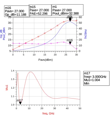
 PERFORMANCE PARAMETERS FOR COMMON SOURCE PA

In the figures below following results are achieved at 3.2 GHz with 27dBm input drive signal.

Output Power = 32.38 dBm Power added efficiency=52.23 %

Power Gain=11.18dB

Optimum Load= 36.1+j13.4 Ohm

[image:32.595.114.491.271.664.2]

Figure 4.4: Performance results of unmatched common source PA

m1 Pavs=

Pout_dBm=32.388 27.000 m15

Pavs= PAE=52.296

27.000 m16

Pavs=

Gp_dB=11.188 27.000

5 10 15 20 25

0 30

10 15 20 25 30

5 35

10 20 30 40 50

0 60

Pavs(dBm)

P

out

_

d

B

m

m1

PA

E(

%)

m15

Gp

_d

B

m16 m1

Pavs=

Pout_dBm=32.388 27.000 m15

Pavs= PAE=52.296

27.000 m16

Pavs=

Gp_dB=11.188 27.000

m17 freq= Mu1=1.004 Min

3.000GHz

10 20 30 40

0 50

1.1 1.2 1.3

1.0 1.4

freq, GHz

Mu

1

m17

m17 freq= Mu1=1.004 Min

(33)

[image:33.595.173.342.533.706.2]

33

Figure 4.5: Frequency (in GHz) characteristic of Pout and PAE for the common source stage

PA

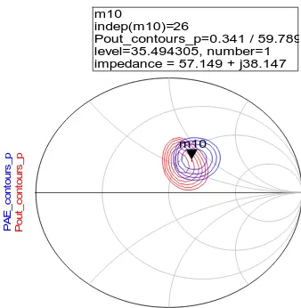
4.1.1 STACKED CONFIGURATION BIASED IN CLASS AB-MODE

As for the single stage, after determining the DC bias condition, the next step was determining the optimum load to be presented to output of transistor. For the cascode configuration we have found Zopt= 57.149+j*38.147

Figure 4.6: Load Pull analysis result of stacked configuration

m3 RFfreq= PAE=51.230 2.700E9 m12 RFfreq= PAE=49.980 4.000E9 m13 RFfreq= PAE=51.158 3.700E9

2.6E9 2.8E9 3.0E9 3.2E9 3.4E9 3.6E9 3.8E9

2.4E9 4.0E9 46 47 48 49 50 51 52 53 54 45 55 RFfreq PAE m3 m12 m13 m3 RFfreq= PAE=51.230 2.700E9 m12 RFfreq= PAE=49.980 4.000E9 m13 RFfreq= PAE=51.158 3.700E9 m1 RFfreq= Pout_dBm=32.142 2.500E9 m10 RFfreq= Pout_dBm=32.066 3.700E9 m11 RFfreq= Pout_dBm=31.812 4.000E9 2.6E9 2.8E9 3.0E9 3.2E9 3.4E9 3.6E9 3.8E9

2.4E9 4.0E9 30.5 31.0 31.5 32.0 32.5 30.0 33.0 RFfreq P out _dB m m1 _m10 m11 m1 RFfreq= Pout_dBm=32.142 2.500E9 m10 RFfreq= Pout_dBm=32.066 3.700E9 m11 RFfreq= Pout_dBm=31.812 4.000E9

indep(Pout_contours_p) (0.000 to 62.000)

P o u t_c ont our s _ p m10

indep(PAE_contours_p) (0.000 to 52.000)

P A E _ c ont our s _ p m10 indep(m10)=

Pout_contours_p=0.341 / 59.789 level=35.494305, number=1 impedance = 57.149 + j38.147

(34)

34

Figure 4.7: Unmatched stacked class AB PA

Figure 4.8: Unconditional stability, K>1 and ∆ 1 is satisfied

Vg1 Vground

Vd Vg

Vin vload

PRC

PRC1

C=50 pF {t} R=25 Ohm {t} VAR

STIMULUS

Vg=-1.6V Vd=28 V RFf req=3.2 GHz Pav s=27_dBm

EqnVar V_DC

SRC1 Vdc=10 V

R

R2 R=100 Ohm {-t}

R

R1 R=100 Ohm {-t}

V_DC V_g Vdc=Vg

C

C2 C=3 pF {-t}

Term

Term3

Z=57.14+j*38 Num=2 F4

PP50_20_TNO_8x250um_v1_1

F3 I_Probe

Iin

P_1Tone PORT1

Freq=RFf req P=dbmtow(Pav s) Z=Z_s Num=1

DC_Block

DC_Block3

I_Probe Ig1

DC_Block

DC_Block2

DC_Feed

DC_Feed3 I_Probe

Ig V_DC

Vground Vdc=0

I_Probe Iload

V_DC V_d Vdc=Vd I_Probe Id

DC_Feed

DC_Feed1

10 20 30 40

0 50

10 20 30 40

0 50

freq, GHz

St

a

b

F

a

c

t1

m3

M

a

g

_de

lt

a

m2 m3

freq=

StabFact1=1.042 Min

1.300GHz m2_freq=

Mag_delta=0.845 Max

(35)

35

Figure 4.9: Source and Load stability Circles

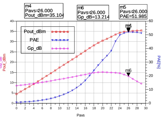
Figure 4.10: Power performance of the stacked amplifier @ 3.2GHz and VDD=28[V]

indep(S_StabCircle1) (0.000 to 51.000)

S_

S

ta

b

C

ir

c

le

1

indep(L_StabCircle1) (0.000 to 51.000)

L_

S

tab

C

irc

le

1

m4 Pavs=

Pout_dBm=35.10426.000

Pout_dBm

PAE

Gp_dB

m5 Pavs=

PAE=51.98526.000

m6 Pavs=

Gp_dB=13.21426.000

2 4 6 8 10 12 14 16 18 20 22 24 26 28

0 30

5 10 15 20 25 30 35

0 40

10 20 30 40 50

0 60

Pavs

P

o

ut

_d

B

m

m4

P

AE[

%

]

m5

Gp

_

d

B

m6 m4

Pavs=

Pout_dBm=35.10426.000

Pout_dBm

PAE

Gp_dB

m5 Pavs=

PAE=51.98526.000

m6 Pavs=

[image:35.595.173.456.396.605.2]

(36)

36

[image:36.595.146.494.116.328.2]

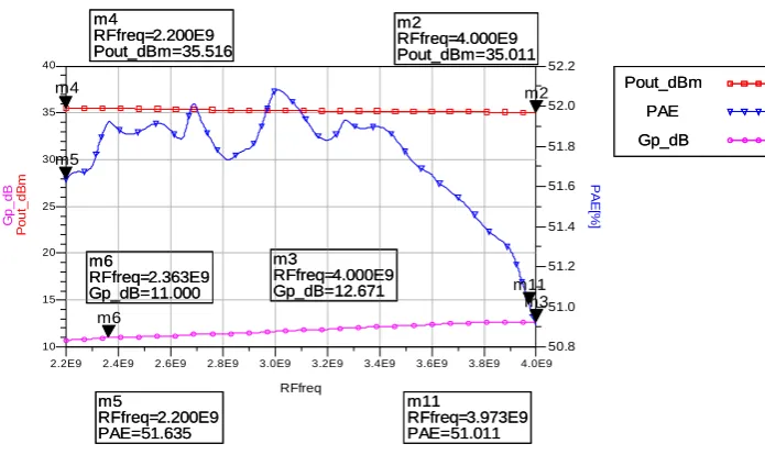
Figure 4.11: PAE, Pout and Power gain versus Frequency of the cascode stage amplifier @ S band

4.1.2

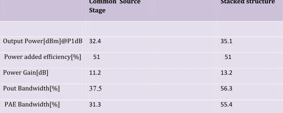
PERFORMANCEOFDESIGNEDUNMATCHEDCLASSABPA

The performance comparison of common source stage ‘linear’ PA with stacked PA is given in table 4.1

The output power is increased almost 2 times in stacked topology compared to the common source stage as expected from the literature information. Other important points are the increased output power bandwidth and PAE bandwidth (about 20% increasing) along with increased power gain in stacked topology.

m4 RFfreq=

Pout_dBm=35.516 2.200E9

m5 RFfreq= PAE=51.6352.200E9 m6

RFfreq= Gp_dB=11.000

2.363E9

m2 RFfreq=

Pout_dBm=35.011 4.000E9

m11 RFfreq= PAE=51.0113.973E9 m3

4.000E9

Pout_dBm PAE Gp_dB

2.4E9 2.6E9 2.8E9 3.0E9 3.2E9 3.4E9 3.6E9 3.8E9

2.2E9 4.0E9

15 20 25 30 35

10 40

51.0 51.2 51.4 51.6 51.8 52.0

50.8 52.2

RFfreq

P

o

ut

_dB

m

m4 _m2

PAE[

%

]

m5

m11

Gp

_

d

B

m6

m3 m4

RFfreq=

Pout_dBm=35.516 2.200E9

m5 RFfreq= PAE=51.6352.200E9 m6

2.363E9

m2 RFfreq=

Pout_dBm=35.011 4.000E9

m11 RFfreq= PAE=51.0113.973E9 m3

4.000E9

(37)

[image:37.595.66.530.25.211.2]

37 Table 4.1: Performance summary of common source ‘linear’ PA and Stacked PA

In the next section we will deal with the same analysis but this time we will do it for a switch mode PA.

4.2

SWITCH MODE DESIGN AS AN ALTERNATIVE APPROACH TO LINEAR DESIGN IN ORDER TO IMPROVE THE EFFICIENCY

Switching-mode power amplifiers (SMPA) use active transistors as switches. That is, the active device is ideally fully on (short-circuit) or fully off (open-circuit). The theoretical efficiency of the SMPA’s is 100%. However this is in practice never the case. Especially in the high frequency range, optimum drain current and voltage waveforms deviate substantially from the ideal non-overlapping situation.

We will perform some simulations with a class E power amplifier with quarter wave transmission line configuration. The reason of chosen configuration is explained in section 4.2.2.4. But it could be also done in other kind of configuration of class E PA.

Common Source Stage

Stackedstructure

Output Power[dBm]@P1dB 32.4 35.1

Power added efficiency[%] 51 51

Power Gain[dB] 11.2 13.2

Pout Bandwidth[%] 37.5 56.3

(38)

4.2.1SI

As to ai class E

F

INGLESTAG

[image:38.595.76.575.155.533.2]

im to increa PA with qu

Figure 4.12:

GECLASS–E

ase the PAE uarter wave

: Single stag

[email protected]

along with transmissio

ge class E po

Z

h output pow on line whic

ower amplif

wer using st ch is given b

fier with qu

ack structur below in the

uarter wave

re, we desig e figure 4.12

transmissio

38 gned a

2

(39)

39

Figure 4.13: Unconditional stability verification

Figure 4.14: Load and Source stability Circles

m2 freq=

StabFact1=1.533 Min

50.00GHz

10 20 30 40

0 50

10 20 30 40

0 50

freq, GHz

St

a

b

F

a

c

t1

m2 m2

freq=

StabFact1=1.533 Min

50.00GHz m3freq=

Mag_delta=1.000 Max

0.0000Hz

10 20 30 40

0 50

0.5 0.6 0.7 0.8 0.9

0.4 1.0

freq, GHz

M

a

g

_del

ta

m3 m3 freq=

Mag_delta=1.000 Max

0.0000Hz

L

_

S

ta

bC

ir

c

le1

indep(S_StabCircle1) (0.000 to 51.000)

S

_

S

tabC

ir

c

(40)

40

[image:40.595.107.450.101.380.2]

Figure 4.15: Simulated PAE, Pout, and Power Gain vs. frequency bias (Vd=10 [V], Vg=-1.75[V]

Figure 4.16: Drain Voltage and current vs. time and load signal vs. time

As it can be seen from the figures 4.13 and 4.14 unconditional stability is satisfied( Rollett stability criteria has been fulfilled). Also from figure 4.16 we observe that the optimum class E condition is not satisfied but further improvement of this condition would make the

bandwidths for output power and PAE much narrower which would be also an unwanted situation moreover the aim of this project is not to desing a best perfomed PA at S band but

2.6E9 2.8E9 3.0E9 3.2E9 3.4E9 3.6E9 3.8E9

2.4E9 4.0E9

5 10 15 20 25 30

0 35

30 40 50 60

20 70

RFfreq

PA

E[%]

m11 m12

Po

ut_

d

B

m

m9 m10

Gp_d

B

m13

m11 RFfreq= PAE=60.355

2.990E9 m12RFfreq=

PAE=60.612 3.320E9 m9

RFfreq=

Pout_dBm=30.523

2.500E9 m10

RFfreq=

Pout_dBm=30.004 3.090E9 m13

RFfreq=

Gp_dB=14.274 Max

2.970E9

0.2 0.4 0.6 0.8 1.0 1.2 1.4 1.6 1.8

0.0 2.0

5 10 15 20

0 25

0.0 0.1 0.2 0.3 0.4 0.5

-0.1 0.6

time, sec

ts

(V

d

in

t[0

,::])

ts(

-I

d

in

t.i

[0

,::]

)

0.2 0.4 0.6 0.8 1.0 1.2 1.4 1.6 1.8

0.0 2.0

-10 -5 0 5 10

-15 15

time, sec

ts

(v

load[

0

(41)

to show this resu

4.2.2ST

Below t compare

In figur in these

w the benefit ult and go fu

TACKEDSW

the stacked e the perfor

e 4.18 the lo e figures tha

ts of cascod further with

WITCHMODE

version of t rmance of si

Figure 4

oad and sou at the uncon

de structure cascode con

EDESIGN

the previous ingle stage w

4.17: Stacke

urce stability ditional stab

at high freq nfiguration

s class E PA with cascod

d Switch mo

y circles alo bility is sati

quencies.So of this clas

A is given. de version o

ode PA

ong with Ro isfied.

it is decide s E PA.

This circuit of the SMPA

ollet’s criter

ed to satisfy

t will be use A.

rion given. W

41 y with

ed to

(42)

42

Figure 4.18: Unconditional stability verification; above the load and source stability circles beneath that

[image:42.595.118.473.101.377.2]

the K factor and Δ are given

Figure 4.19: Drain current and Voltage waveforms of bottom and top transistors indep(S_StabCircle1) (0.000 to 51.000)

S_ St a b C ir c le 1

L_ S ta b C ir c le 1 m4 freq= StabFact1=15.570 26.20GHz m9 freq= StabFact1=4.108 Min 4.300GHz

10 20 30 40

0 50 10 20 30 40 0 50

f req, GHz

S tabF ac t1 m4 m9 m4 freq= StabFact1=15.570 26.20GHz m9 freq= StabFact1=4.108 Min 4.300GHz m12 freq= Mag_delta=0.911 Max 19.70GHz

10 20 30 40

0 50 0.2 0.4 0.6 0.8 0.0 1.0

f req, GHz

M ag_ delt a m12 m12 freq= Mag_delta=0.911 Max 19.70GHz

0.2 0.4 0.6 0.8 1.0 1.2 1.4 1.6 1.8

0.0 2.0 2 4 6 0 8 0.0 0.1 0.2 0.3 -0.1 0.4 time, sec ts (F 3 .V d in t[ 0 ,: :]) ts (-F 3 .Id in t.i [0 ,::] )

0.2 0.4 0.6 0.8 1.0 1.2 1.4 1.6 1.8

(43)

43

Figure 4.20: PAE, Power Gain and PAE vs. Pavs

Figure 4.21: Pout and PAE vs. frequency( in GHz) characteristic

2 4 6 8 10 12 14 16 18 20 22 24 26

0 28 0 5 10 15 20 25 30 -5 35 10 20 30 40 50 0 60 Pavs Po ut _dB m m15 PAE[ % ] m14 G p_dB m17 m15 Pavs= Pout_dBm=33.51923.000 m14 Pavs= PAE=56.909 23.000 m17 Pavs= Gp_dB=15.843 23.000 Pout_dBm PAE Gp_dB m3 RFfreq= Pout_dBm=31.957 2.500E9 m16 RFfreq= Pout_dBm=32.906 4.000E9 m13 RFfreq= Pout_dBm=33.517 3.200E9 m20 RFfreq= Pout_dBm=33.2632.900E9 m21 RFfreq= Pout_dBm=33.349 3.900E9

2.6E9 2.8E9 3.0E9 3.2E9 3.4E9 3.6E9 3.8E9

2.4E9 4.0E9 26.5 28.0 29.5 31.0 32.5 34.0 25.0 35.0 RFfreq P ou t_ dB m m3 m16 m13 m20 m21 m3 RFfreq= Pout_dBm=31.957 2.500E9 m16 RFfreq= Pout_dBm=32.906 4.000E9 m13 RFfreq= Pout_dBm=33.517 3.200E9 m20 RFfreq= Pout_dBm=33.2632.900E9 m21 RFfreq= Pout_dBm=33.349 3.900E9 m7 RFfreq= PAE=57.025 Max 3.300E9 m18 RFfreq= PAE=53.742

2.900E9 m19_RFfreq=

PAE=55.413 3.900E9 m22 RFfreq= PAE=56.918 3.200E9 2.6E9 2.8E9 3.0E9 3.2E9 3.4E9 3.6E9 3.8E9

2.4E9 4.0E9 45 50 55 60 40 65 RFfreq PA E m7 m18 m19 m22 m7 RFfreq= PAE=57.025 Max 3.300E9 m18 RFfreq= PAE=53.742

2.900E9 m19_RFfreq=

(44)

44

4.2.3

PERFORMANCESUMMARYOFDESIGNEDSWITCHMODEPA

In table 4.2 the performance comparison of single stage SMPA with stacked version given. We see here again an increase in the bandwidth and the output power for the stacked topology. Also the power gain is greater for the stacked configuration as it was the case for linear PA.

Table 4.2: Performance summary of single stage SMPA with stacked SMPA

The increase in bandwidth for PAE is pretty high but this is due to the fact that we have used here class E power amplifier with quarter wave transmission line that possess 4 harmonic termination which makes the output characteristics more selective for single stage SMPA. We do not expect that much increasing in the bandwidth for other kinds of class E PAs but still the increasing would be about 2 times more for stacked topology compared to the single stage.

Another important observation is that the switch mode PAs do not perform very well in the sense of PAE and output power when we compare it with ‘linear’ PAs at S band. This is because of the difficulties in achieving the optimum class E conditions at high frequencies. The maximum output power that is achieved with SMPA is almost 2 dBm less than linear PA but it also provides 3dB more output power when using stacked structure compared to single stage version as it was for the linear PA.

In the figure below we see the improvement in the bandwidth characteristic for the SMPA

SingleStage CascodeStage

Output Power[dBm]@P1dB 30.5 33.3

Power added efficiency[%] 60 55

Power Gain[dB] 14.3 15.8

Pout Bandwidth[%] 15.6 31.2

(45)

45

[image:45.595.97.452.103.411.2]

Figure 4.22: Improvement in the bandwidth characteristic for the SMPA: first two belong to the single stage

SMPA and below that the cascode stage SMPA frequency characteristic.

Having finishing the comparison of unmatched circuit performances, it is now time to design the impedance matching circuits for the PAs in order to have a more realistic performance merits.

4.3

IMPEDANCE MATCHING NETWORK DESIGN FOR LINEAR POWER AMPLIFIER

Matching networks provide a transformation of impedance to a desired value to maximize the power dissipated by a load. The input impedance of the transistor is highly nonlinear, i.e., dependent on the operating point. Thus, the device operating under large-signal conditions

2.6E9 2.8E9 3.0E9 3.2E9 3.4E9 3.6E9 3.8E9

2.4E9 4.0E9

45 50 55 60 65

40 70

RFfreq

PAE

2.6E9 2.8E9 3.0E9 3.2E9 3.4E9 3.6E9 3.8E9

2.4E9 4.0E9

28 29 30 31

27 32

RFfreq

P

ou

t_

dB

m

2.6E9 2.8E9 3.0E9 3.2E9 3.4E9 3.6E9 3.8E9

2.4E9 4.0E9

26.5 28.0 29.5 31.0 32.5 34.0

25.0 35.0

RFfreq

P

o

ut

_dB

m

2.6E9 2.8E9 3.0E9 3.2E9 3.4E9 3.6E9 3.8E9

2.4E9 4.0E9

50 60

40 70

RFfreq

(46)

(and esp Therefo As expl counterp matchin

4.3.1IN

After co the f0 of

transfor

Through of ZLopt=

network

In the fi the outp

pecially in s ore it is one lained in sec

part. Theref ng networks

NPUT/OUTP

onnecting th f 3.2 GHz. W rms 50ohm

h load Pull =36,108+j1 k match circ

Output

igure below put and inpu

switched-mo of most imp ction 4.2.3 t fore we will s for this PA

PUTMATCHI

he load netw We then des Zsource into Z

analysis the 3.415 for th cuit that wil

t matching

[image:46.595.74.521.445.708.2]

w, the concep ut of the circ

Figure 4

ode PAs), w portant step the perform l focus on th A.

INGCIRCUIT

work we wil sign a lowp Zin* at f0=3.

e optimum o he common ll transform

circuit Des

ptual design cuit.

4.23: PA wit

will exhibit ps in the des mance of SM he ‘linear’ P

TDESIGNFO

ll determine pass impedan

.2 GHz

output powe n source clas

50 Ohms to

sign for com

n schematic

th input/outp

Zin

Z*in

dynamicall sign of a PA MPA at S ban

PA and desi

ORCOMMON

e the large-s nce transfor

er was deter ss AB PA.

o the optim