Non invasive imaging with UWB

(1)

University of Twente

Department of Electrical Engineering Telecommunication Engineering Group

Non-invasive imaging with UWB

by

Michael Kort¨um

Master thesis

Executed from September 2010 to June 2011

Supervisor: Prof. dr. ir. ing. F. B. J. Leferink Advisors: Dr. ir. M. J. Bentum

(2)

(3)

Summary

Cancer is the main killing disease and breast cancer is the most common tumor among women. Compared to other cancers, the survival rate in case of breast cancer is high when detected early. Therefore intense screening programs are initiated. The standard for detection of breast cancer is mammography, which has several disadvantages such as ionizing radiation, high false-positive and false-negative rates. Ultrasound or magnetic resonance imaging can be applied to find tumors too, but both are not suited for large-scale screenings. Researchers at Dartmouth college have shown that ultra-wideband (UWB) can be a solution as a complementary method. However, the principles on which their prototype relies are not explicitly mentioned. Their applied frequency range of 300 MHz to 3 GHz is not the one ruled by the Federal Communications Com-mission (FCC) or European Telecommunications Standards Institute (ETSI). The FCC ruled that UWB has to operate roughly in the band of 3.1 to 10.6 GHz, whereas the European regulation is somewhat more limited. The aim of this master thesis is to experimentally verify whether medical imaging is possible at the frequencies ruled by the FCC for UWB, whereas the power limitation was not taken into account.

For imaging objects, such as human tissues, different means are needed. The permittiv-ity of a tissue depend on frequency and on the type of tissue. To measure the frequency dependence a means for illumination is needed. UWB is such a means that has several advantages. The large bandwidth of UWB provides good resolving of multipath and (partly) penetration of tissues is possible. Also lesions and noncalcified tumors can be detected by UWB because of their different nature. Regions that are dense and firm can be imaged, such as in the near of the chest wall or underarm. However, UWB has a trade-off between high resolution and maximum penetration depth. Because no equipment was available to use pulsed UWB signals, in this research a swept narrow-band approach is used to experimentally verify whether imaging at the frequencies of UWB is possible. Illuminating the tissue with UWB, scattered fields can be measured applying an array of antennas. These scattered fields can be mapped to an image, showing object shapes and their permittivities.

Every tissue has a different amount of fluid content, by which their frequency behav-iors differ. Using the parametrization given by Gabriel et al. [1]–[3], these theoretical

(4)

curves can be compared to the measured ones. By this it can be identified what is imaged, and even more, it can be determined whether the measured tissue is benign or malignant. The reason is the high difference in permittivity between benign and malignant tissues, persisting over the whole frequency region of UWB. To be able to distinguish the different tissues a wide range of frequencies is necessary to have enough information, because different tissues might have the same characteristics at certain frequencies. It is reasonable to use a means, such as UWB, that has these wideband characteristics. Moreover, its wideband nature provides good resolution capabilities.

To map the scattered fields to an image an algorithm is needed. Due to the high contrast between benign and malignant tissues strong scatterers have to be measured, by which an iterative procedure is used. The iterative process matches the calculated data and the measured fields with each iteration by which it can be applied for high contrasts too. To calculate the fields finite points are needed. That is why the area of interest is subdivided into a mesh. In this thesis a two-dimensional Cartesian mesh is chosen for proving the concept. This two-dimensional mesh remains intuitive and is easy to implement.

The measurement setup, consisting of a network analyzer (for sweeping the frequency), coaxial cables and self-designed log-periodic antennas, is tested by measurements. Us-ing salt solutions, which are frequency-dependent, and by changUs-ing the position of the objects the concept was tested. The accuracy of the measurements and systematic errors were determined. Measurements have shown that the setup is suited. Several objects were measured with an antenna array to calculate images afterwards. From this it can be concluded that different materials can be identified regarding their per-mittivity, and the shapes of the objects were apparent. Increasing the number of views measured and segments of the mesh led to more detailed information of the measured area. Afterwards it was experimentally shown that abnormalities can be recognized.

From the experimental verifications is expected that imaging with UWB will be pos-sible and that tumors or lesions can be recognized. Also the high contrast between benign and malignant tissues is expected to be resolvable, because in this thesis high contrasts were measured too. However, comparing these conclusions to the prototype of Dartmouth college is difficult. They used real breasts and imaged different types of tissues at the same time, whereas in this thesis only one tissue was measured. For comparison more information about the prototype of Dartmouth college is needed. The used antennas in this thesis could have been improved and calibrated, the measure-ments could have been done in an anechoic chamber, an antenna array could have been built and the algorithm could have been optimized. Still a system has to be designed and developed in future. For this it has to be researched whether UWB indeed can be used at these frequencies and requirements have to be formulated.

(5)

CONTENTS v

List of acronyms

ETSI European Telecommunications Standards Institute

FCC Federal Communications Commission

LPDA log-periodic dipole array antenna

MFLOPs mega floating-point operations

MRI magnetic resonance imaging

OUT object under test

PET polethylene terephtalate

PSD power spectral density

TM transverse magnetic

UWB ultra-wideband

(8)

(9)

Chapter 1

Introduction

1.1

Motivation

Nowadays cancer is one of the main killing diseases in the society. Around 25 % of yearly deaths are caused by cancer [4]. The most common tumor found among women is breast cancer, as reported by the World Health Organization [4], [5]. Worldwide, breast cancer is the most frequent kind of tumor among women with 23 % of all stated types of cancer. This type of cancer leads to 30 caused deaths in a population of 100,000 every year [4], [6]. The number of new breast cancer patients reported was around 1.15 million cases in 2002. That is why breast cancer got the second rank of all types of cancer behind lung cancer, when both sexes are considered [4]. Moreover, one out of eight women will get cancer during their life [7].

In a global average the survival rate of breast cancer is 65 % [4], [6]. As can be noted by this, breast tumors have a good survivial rate when detected early enough compared to other forms of cancer. Therefore screening programs are initiated that are carried out in the developed countries [4], like the US or in Europe. They are established especially to find invasive tumors in an early state. However, breast cancer still causes 411,000 deaths in the developed countries annualy, as was reported in 2002 [4], [6]. Also the occurrence of breast cancer is still increasing in most countries. Even more tremendous is that the breast cancer rates increase where they were previously low. In East Asia the growth is estimated with 3 %, whereas it approximately increases by 0.5 % in the rest of the world [4]. Consequently the world total would be around 1.5 million breast cancer patients in 2011 [4], [6].

The reason for the screening programs in the developed countries is that there is a strong correlation between the clinical outcome of breast cancer and the size of it when it is detected. The chance that a person survives can be estimated from the size of the

(10)

2 Chapter 1. Introduction

tumor independent from the method of detection [8]. That is why in most developed countries women frequently have to visit their radiologists.

Moreover, visiting the screening programs is necessary because getting breast can-cer is unpredictable. It can be the case that women that have many breast cancan-cer risk factors do not develop it. This can also be the other way around, that a woman that may be considered at low risk will get a positive result [7], [9].

Nowadays, the standard technique used is mammography to detect malignant breast tumors. This technique has several disadvantages, such as that ionizing radiation is used. This radiation could potentially also induce cancer into the patient, even if the level is kept as low as possible. It has been shown that women passing an X-ray during 10 years have a chance of eight out of 100,000 to die [4], [10]. Comparing this to the number of deaths caused by breast tumors this is still a high amount (which is 30 out of 100,000).

Moreover, the false-positive rate of mammography is estimated to be between 2.8 % and 15.9 %, whereas there is the chance of a false-negative result of 4 % to 34 % [4], [11], [12]. These false rates are especially dependent on the experience of the radiolo-gist. After a mammography, still 10 % to 50 % [4], [13] of the women need a biopsy to verify the findings made by the mammogram. It can also be the case that breast cancer is not detected by the mammogram, which is the result in 5 % to 15 % of the screenings [4], [11], [12]. The reason for this is that it is difficult to image radiographi-cally dense breasts [4], [13]. In that case there is a high content of fibrous and glandular tissues which are soft ones such as breast cancer. Consequently the contrast between malignant and benign tissues is very low in X-ray mammography [12], [14]. If it can-not be concluded whether there is a tumor present, alternative imaging techniques are applied [13].

(11)

More-1.1. Motivation 3

over, the patient is not allowed to move because otherwise the whole image has to done again [17]. That is why this method is not suited too.

The highest detection rates of breast cancer are reported in developed countries, be-cause of the intense screening programs [6]. This changes dramatically in lower devel-oped countries, such as in Africa. There the same rates of mortality caused by breast cancer are reported, but the detection rates are very low. That is why a cheap, sen-sitive and accurate method has to be found so that it also can be used within lower developed countries.

From the previous discussion it follows that there is a high need for a complementary method to detect breast cancer, to be able to decrease the worldwide mortality rate. For this ultra-wideband (UWB) imaging can be the solution, as shown by the clinical prototype developed at Dartmouth college [20], [21]. They use the frequency range of 300 MHz to 3 GHz to create two-dimensional images by the data sets obtained from an antenna array. For that they use presumably the tomographic imaging approach, which needs 14 minutes for imaging both breasts. However, within their work they only state what the prototype looks like and which results they achieved. The principles on which the prototype relies and whether they satisfy the power limitations of UWB is not described explicitly. Presumably, they used the fact that there is a difference in between benign and malignant tissues.

(12)

4 Chapter 1. Introduction

According to the literature, using UWB for medical imaging is still a challenge, because of [26]–[30]:

• the human being in the near field of the antennas most of the time;

• mutual coupling between the antennas;

• resolving the inverse scattering problem in an exact way;

• optimization of computationally expensive large linear systems;

• calculation results that are very sensitive to noise in the measured data.

Still there is much ongoing research on this topic to find the right coupling medium to decrease the mutual coupling and reflections from the air/skin boundary. Also optimizing the inversion algorithms is further researched to image as fast as possible. However, for this fast processors are needed which have improved their speed more and more during the last years.

1.2

Objective of the assignment

In this master thesis a similar method to the one of the prototype of Dartmouth college is used. However, in this thesis is investigated whether UWB in the frequency range of 3 to 10 GHz is suitable for medical imaging and cancer detection. This raises the following research question:

• Can the frequency band determined by the FCC for UWB be used for medical imaging?

1.3

Report organization

(13)

Chapter 2

Needs for imaging

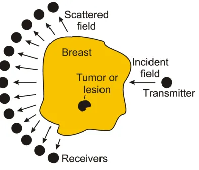
[image:13.595.217.414.544.713.2]

In this chapter the three parts, which are needed for imaging an object under test (OUT), are discussed. The internal structure of an object can be measured with the use of electromagnetic fields at microwave frequencies (300 MHz to 30 GHz) [31]. The electric field is affected by the tissue. The setup for measuring is shown in Figure 2.1. There a transmitter is used to illuminate the breast using UWB. The wave travels through it and can be detected by receivers located at the opposite side. If an abnor-mality (like a tumor or lesion) is present (as depicted in Figure 2.1), the waves will encounter a change in their properties on the way through the breast. The incident wave is scattered and the amount of energy collected by the antennas changes [31]. Using this information about the scattered energies an image can be formed. The first part is the affect of the tissue on the electric field, which is described in Section 2.1. In Section 2.2 the illuminating technique UWB (the second part) will be discussed. Finally, the last part, represented by the imaging principle is treated.

Figure 2.1: The basic microwave imaging problem with a tumor present.

(14)

6 Chapter 2. Needs for imaging

2.1

Behavior of tissue in an electric field

An electric field is affected by the biological tissue [32]. The tissue can be described by the permittivity .

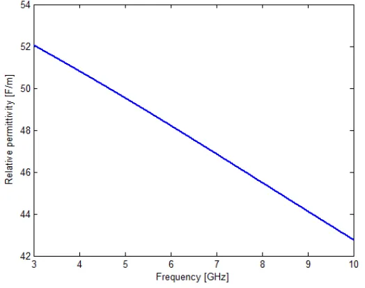
[image:14.595.154.416.268.475.2]

In any heterogeneous material, also in biological tissue, dispersion can be found [32]. Figure 2.2 shows the typical dispersion for the UWB region related to the variation with frequency of the permittivity. As shown, the permittivity is frequency-dependent and decreases with frequency. The dispersion at these frequencies is caused by the polarization of the water molecules inside the materials [32], [33].

Figure 2.2: Typical frequency dependence of the permittivity of a heterogeneous material such as biological tissues.

Every biological material has different frequency dependencies, as will become clear in Chapter 3. This difference can be used to determine exactly which type of tissue was measured. However, to generate a curve of the measured permittivity for comparison with known tissue graphs, a wide range of frequencies has to be applied to get enough information. To get a wide range of frequencies it is reasonable to use a technique that has these wideband characteristics. UWB is such a technique, which has additional advantages.

2.2

UWB

(15)

2.2. UWB 7

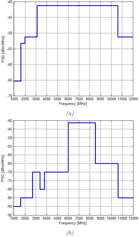
6 to 8.5 GHz can be used with a PSD of ₋41.3 dBm/MHz [23], [24]. The maximum emission limits according to the FCC [22] and ETSI [23], [24] are shown in Figures 2.3a and 2.3b, respectively.

(a)

[image:15.595.199.426.164.551.2]

(b)

Figure 2.3: Maximum emission or PSD (a) according to the FCC and (b) according to ETSI.

UWB systems are also cheap and less complex compared to traditional narrowband systems. The reason is that, within UWB systems, a short pulse of less than a nanosec-ond is generated which can be transmitted at baseband [34], [35]. This principle of transmission needs no up or down conversion as required by narrowband systems.

The large bandwidth of UWB is advantageous to resolve multipath components [34], [35]. By using these short signals many of the narrow pulses can be resolved indepen-dently instead of being combined destructively.

(16)

8 Chapter 2. Needs for imaging

human tissues [34], [35]. However, there is a trade-off between high resolution and maximum penetration depth. Attenuation of the signals comes important in imaging humans because of the high water content of tissues. The attenuation quickly increases with frequency. At a frequency of 1 GHz the attenuation equals 0.2 to 0.5 dB/cm, which changes to 0.5 to 30 dB/cm at 10 GHz [36].

Another advantage of UWB is its possibility to detect lesions as well as noncalci-fied cancer [37]. This is valid for all microwave techniques up to 11 GHz, as will be discussed in Chapter 3. Moreover, with UWB it is possible to detect tumors in dense breasts. Also regions near the chest wall or underarm [37] can be imaged, which are firm and dense because there are many layers of tissue above each other.

From these advantages and its ability to operate non-invasively and being biologi-cally friendly, UWB has many positive features for medical imaging. Still it has to be researched whether it is user-friendly and technically understandable by the radiolo-gist, and has high sensitivity and high accuracy [38].

During this research work it was not possible to generate, to shape and to receive a pulsed UWB signal, because the equipment was not available. Therefore an approach was chosen in which the signal is swept over the frequency band of 3 to 10 GHz. That is why in this thesis it is verified whether imaging at the frequencies used by UWB is possible or not. Whether a UWB signal at the frequencies ruled by the FCC can be used for imaging under the power limitations (shown in Figure 2.3a) is beyond the scope of this thesis.

2.3

Tomographic imaging

As already described in the beginning of this chapter, one antenna is used to transmit and numerous antennas surrounding the object to receive the scattered waves. Af-terwards, the position of the transmit antenna is changed and the whole process is repeated [39]. The object shape and spatial distribution of the dielectric can be eval-uated from these measurements.

(17)

Chapter 3

Tissues

As already mentioned in Section 2.1, miscellaneous types of tissues can be distinguished because of their difference in frequency dependence. These differences are caused by variations of the fluid content of the material [32]. In Section 3.1 the dielectric prop-erties of different types of tissues are treated, together with the Cole-Cole equation that describes this frequency dependence. These curves can be used for comparison to define which type of tissue was measured. Moreover, having such curves it can be analyzed whether the tissue measured is benign or malignant, as will be discussed in Section 3.2.

3.1

Dielectric curves of human tissues

The dispersion is the frequency dependence of the permittivity for different types of tissues (as was described in Chapter 2.1). These different permittivity curves can be approximated by the so-called complex Cole-Cole equation. It is defined as [40]:

c =∞+

s−∞

1 + (jωτ)(1−_α₎ −j

σ0

ω0

(3.1)

The parameterss and∞ refer to the relative permittivities at frequencies well above and below the dispersion region, respectively. The variable σ0 is the conductivity of

the tissue above the dispersion region, α is a parameter that depends on the material and ω is the angular frequency. This permittivity (3.1) can be rewritten in a real part and an imaginary part by which it becomes complex:

c = 0

−j00 =0

−jσ

ω (3.2)

The nominator and denominator of the first fraction of (3.1) has to be multiplied by the transpose conjugate of the denominator, which is 1 + (₋jωτ)(1−α)_{. Writing this}

out the real and imaginary parts of the permittivity according to (3.2) are found. The

(18)

10 Chapter 3. Tissues

real part, describing the relative permittivity r, is then found by [41], [42]:

r =∞+ (s−∞)

1 + (ωτ)(1−α)_{sin (}_απ/₂₎

1 + 2(ωτ)(1−α)_{sin (}_απ/_{2) + (}_ωτ₎2(1−α) (3.3)

The imaginary part that is found by this calculation has not the form that can be found in [32], by which doubts remained whether the equation stated there is consistent. That is why only the permittivity was used in the following of this thesis.

A review of 30 different tissues over a large frequency range can be found in the articles published by Gabriel et al. [1]–[3]. They used the Cole-Cole equation to estimate the dielectric properties for the different tissues. Their developed parametrization can be a help and starting point to get a reasonable estimate of the permittivity at any frequency of UWB for these tissues.

Their parameters are substituted into an equation similar to (3.3) [1]–[3]:

r =∞+

4

X

n= 1

∆n

1 + (ωτ)(1−αn)

sin (αnπ/2) 1 + 2(ωτ)(1−αn)sin (α

nπ/2) + (ωτ)2(1−αn) (3.4)

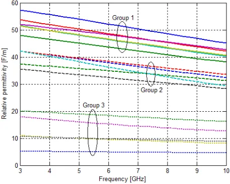
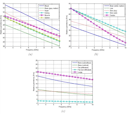
[image:18.595.170.398.466.648.2]

Gabriel et al. measured different types of tissues and developed a parametrization of them. This parametrization is shown in Figure 3.1 for 16 different types of tis-sues [1]–[3]. These can be subdivided into three groups, having high, medium and low permittivity. These three permittivity groups are depicted in Figure 3.1.

Figure 3.1: Permittivity versus frequency of the different types of tissues researched by Gabriel et al.

(19)

3.1. Dielectric curves of human tissues 11

The second group, with intermediate permittivity values, consists of brain (white mat-ter), liver, skin (dry), skin (wet), and tendon. The permittivities of these five tissue types are depicted in Figure 3.2b. As shown in Figure 3.2b, the tissue types liver, wet skin and tendon have the same permittivity at a frequency of 3 GHz. Increasing the frequency they can can be distinguished from each other.

The last group, with the lowest permittivities, consists of bone (cancellous), bone (cor-tical), fat (infiltrated), fat (not infiltrated), and lungs. The permittivities of these five tissue types are depicted in Figure 3.2c. As shown in the figure, the tissue types bone (cortical) and fat (infiltrated) are very close to each other, with which it may be diffi-cult to distinguish them from each other.

(a) (b)

[image:19.595.97.531.312.702.2]

(c)

(20)

12 Chapter 3. Tissues

After calculation of an image these curves of the permittivity can be used to identify the tissue. The area under consideration is discretized by a mesh structure for the imaging algorithm, as will be described in Chapter 4. Several of the segments of the mesh structure are averaged. This is done for multiple frequencies to get several points. Afterwards a line can be drawn through the points to connect them with each other. By this a curve is formed which can be compared to the theoretical data to identify the tissue measured. Knowing the values of the permittivities can also be used for the initial contrast of the algorithm (as will be treated in Chapter 5). It is also possible to define whether the tissue measured is benign or malignant.

3.2

Contrast between benign and malignant tissue

The work done by Chaudhary et al. [43] was directed on the identification of breast cancer among women. They measured the relative permittivity of normal and ma-lignant breast tumors of 15 different patients up to 3 GHz. The same was done by Joines et al. [44] for a frequency until 0.9 GHz. They showed that the permittivity of malignant breast tumors exceeds a contrast (ratio between the permittivities of normal and cancerous tissue) of 3.8:1 at 0.9 GHz. Moreover, they found out that the contrast between malignant and normal breast tissue is the greatest in the case of mammary gland. The data measured by Chaudhary et al. is in good agreement with the ones of Joines et al. Chaudhary et al. measured a permittivity contrast of 5:1 at 3 GHz. This is presumably one of the reasons the group at Dartmouth college started developing a clinical prototype.

Gabriel et al. also made measurements on normal tissue and tumors [1]–[3]. With their measurements they developed a model of the measured curves. They found out that high-water-content tissues (such as malignant tumors) have permittivity of an order of magnitude greater than low-water-content tissues. Their model is plotted in Figure 3.3 to show the contrast difference. Note that the contrast persists over the entire measured frequency spectrum, including the band where UWB is used. Still UWB has the advantage of its wideband characteristic, whereby a large frequency spectrum can be measured to get enough information to distinguish the tissues (as was pointed out in Section 3.1). This may not be possible using a narrowband technique for imaging, looking at Figure 3.2b at a frequency of 3 GHz.

3.3

Conclusion

(21)

3.3. Conclusion 13

Figure 3.3: Comparison of the permittivity of high-water-content tissue (such as a tumor) with low-water-content tissue (such as fat) as a function of frequency.

as described by the Cole-Cole equation, these curves can be compared to measured data. For that it is possible to identify what was measured. Moreover, from this it can be concluded whether the tissue is benign or malignant. The reason is the contrast difference, which persists over the whole frequency spectrum of UWB.

(22)

(23)

Chapter 4

Imaging algorithms

To calculate the permittivity curves shown in the previous chapter, it is necessary to have an algorithm to map the measured electric fields to a permittivity image. There are different techniques, as described in Section 4.1. In Section 4.2 it will be dealt with the reason why the iterative scheme is used. Furthermore, the basic principle of the iterative scheme will be described and which assumptions have to be made for it. Thereafter, in Section 4.3 is treated how the iterative algorithm is implemented.

4.1

Different imaging algorithms

As was pointed out in Section 2.3, the aim of electromagnetic scattering problems is to derive the locations and dielectric parameters of arbitrary objects from measured scattered data. To get an efficient solution for imaging, intensive studies have been performed on the reconstruction algorithms. There are three alternatives that can be applied.

The first one which is suited for UWB imaging is the so-called diffraction tomogra-phy [45]–[47]. The main advantages of this technique are its explicit formulas with which the imaging problem can be solved and its fast numerical algorithms by using fast Fourier transforms [45]. For this technique is assumed that there are weak scat-terers [47], whereby approximations can be used. As long as the first-order Born [48] or Rytov [49], [50] approximations are valid it will work well, otherwise imaging will fail. In this case it will fail, because from Section 3.2 it is known that strong scatterers have to be measured.

The second option is to determine the exact solution of the electromagnetic inverse scattering problem. In literature many different solutions to this nonlinear inverse problem can be found [48], [51]. These solutions are mostly based on moment meth-ods [48], [51]. However, the convergence of these algorithms depends on the contrast

(24)

16 Chapter 4. Imaging algorithms

of the object. The higher the contrast difference, the less likely a solution will be. The reason for this is that these algorithms are sensitive to high contrast differences, measurement inaccuracy and observation positions [52]. This leads to a system of equations which is ill-posed, because small changes in the measured data can lead to large changes in the solution.

This kind of algorithm is only suited for weak scatterers. However, equipping it with an iterative procedure, the third alternative, a solution to the inverse scattering problem for strong scatterers can be found. This iterative process reduces the effect of ill-conditioning significantly. Moreover, it tries to match measured fields and calculated data more and more with every iteration, by which it can be used for every contrast.

4.2

The iterative algorithm

Several variations of the Newton iterative scheme were published [52]–[54]. However, even after some optimizations, published in [55]–[59], these algorithms can only image rather small objects that have dimensions in the order of a few wavelengths of the applied frequency. Using a priori information the convergence process can be made quicker. This information can consist of the external shape of the object, upper and lower bounds of the complex permittivity, or other helpful information [52].

This kind of imaging can be done two- [49], [51]–[59] or three-dimensionally [60]–[62]. Using two dimensions is more intuitive than applying three. Also the algorithm re-mains simpler and is easier to implement. Moreover, fewer measurements are needed (as will become clear from Chapter 5). That is why imaging in this research work is done two-dimensionally. However, in a future system this should be done using three dimensions, because this may be less computational expensive than a layered two-dimensional system. Moreover, using three dimensions not only the contrast of the tissues is apparent, but the form and size of a tumor can be estimated too.

(25)

4.3. Steps to get to an image 17

The incident electric wave at position r generated by the transmit antenna at loca-tion r’ has the following form:

E(r0

) = jωµ0 4π

exp(₋jkb|r−r0|)

|r₋r0

| |PE(ϕ)| (4.1)

The angle ϕ is created in the propagation direction of the wave and µ0 is the

perme-ability in vacuum. The parameter kb is the wave number of the background (in this case air), which can be described by [51]:

kb = r

ω2_µ

00b−j

ωµ0σb

0

(4.2)

The variablesbandσbare the relative permittivity and conductivity of the background medium, and0is the permittivity of vacuum. The magnitude in (4.1) can be described

by [63]:

|r₋r0

|=p(x₋x0

)2_{+ (}_y₋_y0

)2 _(4.3)

The pair (x, y) describes the observation location, whereas (x’, y’) are used for the source points. The pattern function_|PE(ϕ)_| equals the electric far field pattern of the used antenna. Within this research work an LPDA was used, by which the pattern function has the form of (A.16).

For a calculation of finite points of the fields it is necessary that the area under consid-eration has to be discretized by a mesh structure [64]. Consequently the physical wave propagation can be approximated. The discretization can be solved using a Cartesian mesh [51]–[55], [64] or polar mesh [62], [64], [65], or triangles [56] can be applied. The shape of the object is taken to be arbitrary, and because it is more intuitive and simpler to implement, the Cartesian mesh is used (which is shown as an example in Figure 4.1).

Solving the permittivity values inside the mesh can be done by iteratively processing computed or measured data. In this case the scattered power outside the region of interest was measured by applying an array of antennas.

4.3

Steps to get to an image

(26)

[image:26.595.173.397.85.314.2]

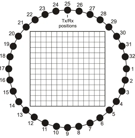
Figure 4.1: The Cartesian mesh surrounded by 32 possible transmitter (Tx) and receiver (Rx) posi-tions. By this 32 transmitter positions 32 views are possible with 13 receive antennas on the opposite side of each transmitter.

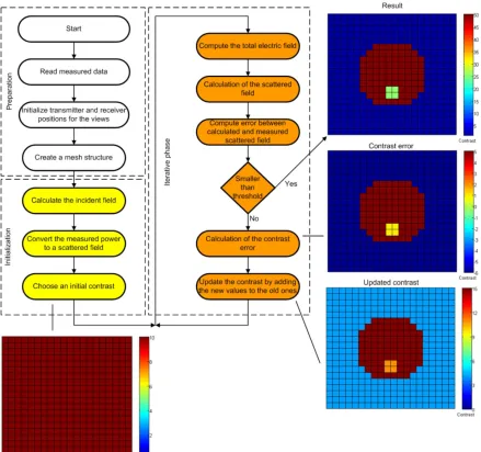
As shown in Figure 4.2, the program starts with the preparation part. There the mea-sured scattered power is read, which was previously stored. This is followed by the definition of the transmitter and receiver positions for the different views (as was shown in Figure 4.1). Thereafter, the mesh structure is created which depicts the calculated permittivity values at the end.

Then the initialization phase is entered. There the incident field of the transmitter is calculated for every segment and each view of the mesh. Looking at Figure 4.1, a view can be described, for example, using position one as transmitter location and at the opposite side the receive antennas are positioned. As shown in that figure there are 32 possible views. Because the measured data consists of the scattered power instead of the field, it has to be converted. An initial contrast is chosen to start the iterative scheme. To explain it more easily, here an initial contrast of 10 was chosen for all segments in a 20_×20 mesh. For the images in Chapter 5 other initial contrasts were chosen, which are presented there.

(27)

[image:27.595.94.533.85.497.2]

4.3. Steps to get to an image 19

Figure 4.2: The flowchart of the iterative algorithm subdivided into the three parts of the initialization, preparation and iterative phase.

In this case an error of 0.5 was selected. This error is large compared to the one found in [52] of 10−₆

(28)

4.4

Conclusion

Having only small contrasts between the different media to be imaged, the diffraction tomography or the inversion algorithm can be applied. However, both are only suited in the case of weak scatterers. The only solution applicable to strong scatterers, which is the case here, is an iterative procedure that is capable to resolve the permittivity profile. The reason is that the calculated fields are iteratively matched to the measured ones. Using the iterative scheme, measurement inaccuracies and high contrasts in the collected data have less influence on the result of the image calculation compared to the former two techniques.

(29)

Chapter 5

Experimental verification

In this chapter it is experimentally verified whether imaging, including cancer identi-fication, at the frequencies of UWB is possible. Consequently the following questions are raised:

• Is imaging of objects possible?

• Can abnormalities be recognized?

In Section 5.1, it is defined by what an answer is found to the questions. Section 5.2 describes the used measurement setup. There it is explained what is used for measuring and how it is implemented. This measurement setup is tested with measurements on the frequency behavior of the used objects, as is treated in Section 5.3. Furthermore, the error that can be introduced into the measurement, when the object is not proper positioned, is estimated. In Section 5.4 an answer to the previous questions is found. There it is dealt with the imaging part which is used to show whether different materials can be identified in an image. Also it is experimentally verified in this section whether it is possible to show abnormalities in the images. Finally, in Section 5.5, the theoretical permittivity curves of the used objects are compared to the measured ones.

5.1

Approach

To verify the questions stated in the introduction, it is started with a test measure-ment to check that the chosen measuremeasure-ment setup (described in Section 5.2) works as expected. For that the frequency dependence of the used salt solutions is measured, together with some evaluations on different positions of the object to determine the errors.

Thereafter, an array is simulated by using one antenna that is shifted between the different receiver positions. The measured data is read by the algorithm described in Section 4.3, to calculate the permittivity profiles for different salt solutions. When this

(30)

22 Chapter 5. Experimental verification

works, it will be experimentally verified whether it is possible to see an abnormality when another object is put into one of the salt solutions.

Finally, the theoretical curves of the calculated salt solutions are compared to the measured ones, that are calculated to have approximately the same permittivity as two tissue types.

5.2

Measurement setup

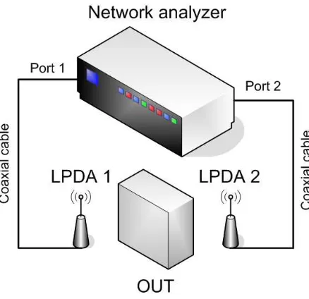
[image:30.595.175.394.451.663.2]

The measurement setup is shown in Figure 5.1. As already mentioned in Section 2.2, a swept narrowband approach instead of the pulsed UWB waveform is used for mea-surement. For that an Agilent PNA-1 network analyzer, having a frequency range of 10 MHz to 20 GHz, and two coaxial cables were used. The frequency of the network analyzer was swept from 3 to 10 GHz. Each of the two coaxial cables was connected to an LPDA. Only two of these antennas were fabricated and used. One acts as the transmit and the other one as the receive antenna. Moreover, the receive antenna is moved between the different receiver positions to simulate an array for the imaging part described in Section 5.4. That is why no mutual coupling between the antennas has been taken into account.

Figure 5.1: The used measurement setup.

(31)

5.2. Measurement setup 23

used antennas are uncalibrated and their patterns or gains remained unknown. That is why the transfer between the antenna terminals including the antennas is measured.

Within this research work only static objects were measured and imaged. Moreover, these measurements were evaluated in a laboratory and not in an anechoic chamber, which has influences on the measurement results (as treated in Section 5.3).

Initially it was considered to place a so-called phantom in between the two antennas, as OUT. These phantoms can be filled with different materials, which have similar properties (especially permittivity) as a human would have. However, this idea was discarded because of the high prices of several thousand of euros [68]–[70]. That is why a cheaper method had to be found, by which the idea of placing different salt solutions in miscellaneous types of bottles was born. More specifically the used salt solutions are so-called sodium chloride (NaCl) solutions. The three different used bottles are shown in Figure 5.2.

Figure 5.2: The three different used OUTs consisting of a PET and two soda-lime glass bottles

The plastic bottle is made of polethylene terephtalate (PET), having a diameter of 8 cm. The other two glass bottles used are made of brown soda-lime glass having diameter of 9.5 cm and 7 cm, respectively. Their capacity can be described by 1.5 l, 1.0 l and 0.5 l of salt solution.

(32)

Before each measurement started, both ports of the network analyzer were calibrated. For that the network analyzer was set to the frequency range of 3 to 10 GHz and an output power of – 5 dBm was used. This output power is the standard one when the device is switched on. The bandwidth used for the measurements had a size of 41.186 MHz, resulting into a PSD of ₋0.1214 dBm/MHz. Calibration was done by measuring opens, shorts and loads connected to the two coaxial cables at both ports. The calibration was finalized by measuring the throughput between the two ports. Again the two coaxial cables were used so that they were not influencing the measure-ment results.

Within the measurements the S12 parameter was measured using the network ana-lyzer. This parameter describes the transfer from antenna 1 to antenna 2. Because uncalibrated antennas were used, also the influences of the antenna and not only the object itself were measured.

5.3

Frequency and position dependence

In this section the measurement setup (introduced in Section 5.2) is tested. For that it is started in Section 5.3.1 with measuring the frequency dependence of the used salt solutions filled into the different types of bottles or even empty OUTs. Furthermore it is tested if it matters to use an object of the same material having different dimensions. In Section 5.3.2 the errors are measured that can be introduced in the measurement when the object is not properly positioned.

5.3.1

Frequency dependence

The first measurement was done using different separations between the two LPDAs. The used separations were 15 cm, 20 cm, 30 cm, 40 cm, 50 cm and 60 cm. For that both antennas were placed on a table and directed towards each other. This is shown in Figure 5.3 for the empty PET bottle. To get these separations most accurate tem-plates were used defining the positions of the antennas and the OUTs. However, small inaccuracies in the order of millimeters could not be avoided because it was not possible to set the antennas exactly on the pre-defined position for every measurement. The measurement was evaluated for an empty space between the antennas and all three OUTs being filled with the salt solutions or empty.

(33)

[image:33.595.185.440.497.700.2]

5.3. Frequency and position dependence 25

Figure 5.3: The two LPDAs separated by a distance of 15 cm having an empty PET bottle in between.

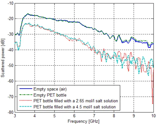
However, it seemed that the multipath components were too strong, resulting in very disturbed measurement results. An example of such a disturbed measurement result is shown in Figure 5.4. In the case of the empty spacing and using an empty PET bottle only small distortions were visible. These disturbances only appeared with the two salt solutions. The reason why these distortions appeared at higher frequencies is because of the weak scattered power from the OUT at these frequencies. Because of the weak scattered power, the multipath components became more dominant. At lower frequencies the scattered power is high enough so that the multipath components are not visible, although they are still there.

(34)

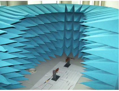
That was the reason why some panels of absorbing material were placed in a half-circle around the receiving antenna (as depicted in Figure 5.5). Hence, most of the multipath components were eliminated. After this conclusion the previous measurements were re-done.

Figure 5.5: Panels of absorbing material placed in a half-circle around the receiving antenna.

[image:34.595.180.390.163.324.2]

A better measurement result with absorbing material for a PET bottle for a separation of the antennas of 20 cm is shown in Figure 5.6. Here the disturbances vanished, and only small distortions remained which could not be avoided. These distortions are still caused by environment. It needed some practice and time to find out the right place for the receive antenna between the absorbers to have as less as possible reflections in the measured signal. It can be concluded that only placing absorbers around the receive antenna results not into ideal measurement results. For that an anechoic chamber might be the better solution.

(35)

The sensitivity of the LPDAs was no solved with the absorbers. Touching the feeding line of the antennas led to differences in the measurements. This might was due to the soldering at the feeding tube of the antennas. It is difficult to solder a cable to a copper tube, which was used for the antennas. To make the soldering as good as possible the coating of the copper tube was filed off, but still the sensitivity remained. It might has been the case that the antennas were mismatched too. The coaxial cable might has not the same impedance as the antennas, even though it was calculated to be.

Increased was this sensitivity effect by the semi-flexible coaxial cables with which the calibration was done. These were connected to the two LPDAs and by this they were dragging on the feeding cable of the antennas. The measurement results were influ-enced much. However, by experimenting with the antennas the best placement of the semi-flexible coaxial cables was found to minimize their influence. This experimenting had cost much time and the influence could not fully be removed.

Taking Figure 5.6 and looking at the curve for the free space measurement, it is shown that the curve increases till 3.9 GHz and thereafter it decreases with frequency until 8.8 GHz. After this it starts increasing again. That it starts increasing at the beginning is most likely due to a dip of the gain. The calculated gain is shown in Figure A.10a and there the dip can be found at 3.5 GHz. Because of the fact that the antennas are manufactured by hand and are not that accurate regarding their dipole positions and lengths, this dip may shifted to a lower frequency. Moreover, it can be that the used equations to design the LPDAs are only suited for free-space.

Moreover, that the curve of the free space measurement in Figure 5.6 is decreasing with frequency after 3.9 GHz is partly caused by the used coaxial cable of the antenna. The used cable is not suited for these high frequencies, because its loss increases with frequency. To show this the measurement setup of Section 5.2 was changed. The two LPDAs were disconnected, and a similar coaxial cable to the one used within the an-tennas was connected to the two calibrated cables and measured. The measured loss of the coaxial cable is depicted in Figure 5.7. For the rest the behavior of the free space curve is not clear, because the characteristics of the two antennas remained unknown.

(36)

[image:36.595.157.413.87.292.2]

Figure 5.7: Measured attenuation of a similar coaxial cable as used within the LPDAs of length 1 m for the applied frequency range in dB/m.

Calculating the difference of the measured result of Figure 5.6 of the empty space and placing an empty PET bottle in between, Figure 5.8 is obtained. The figure shows the additional loss which is due to the PET bottle. The peak around 8.6 GHz is the result of the PET bottle, as results from Figure 5.6. The two peaks in Figure 5.6 are not at the same frequency by which the peak results in Figure 5.8. The reason for this is the bottle itself by which the antennas do not operate at their designed resonance frequencies.

[image:36.595.158.412.498.701.2]

(37)

The difference in loss, that is depicted in Figure 5.8, is frequency dependent, even though the difference in loss between air and PET is small. This difference in loss leads to the conclusion that it might be possible to distinguish between air and PET using images.

Coming back to Figure 5.6, it is shown that the two curves of the bottles filled with the salt solutions are more attenuated than the ones of air or the empty PET bottle. This can be recognized starting at a frequency of 4 GHz. Furthermore, the curves of the salt solutions decrease slightly faster with frequency than the other two. Considering the loss of the different materials, such as air, PET and the salt solutions, the materials can be distinguished from each other. This leads to the conclusion that it might be possible to distinguish these materials in images too.

Even between the two salt solutions a difference in their frequency dependence of their loss can be recognized. The 2.65 mol/l solution is not decreasing as fast as the one of 4.5 mol/l. Such a difference in their frequency dependence is shown in Figure 5.9 for a separation of 60 cm. For that the curve of the 4.5 mol/l solution was subtracted from the other solution graph. That the curve is going up and down is caused by distortions in the measurement results. However, by their different loss characteristics it might be possible to distinguish between the two salt solutions when images are used.

Figure 5.9: Calculated difference in loss between the two salt solutions for a separation of the LPDAs of 60 cm using a PET bottle.

(38)

[image:38.595.172.397.85.268.2]

Figure 5.10: Measurement result of having an empty space, placing an empty soda-lime glass bottle (having diameter of 7 cm) or filled with one of the two salt solutions in between the two LPDAs for a separation of 50 cm.

Still the curves of the two salt solutions decrease faster with frequency than the other ones, as shown in Figure 5.10. From this it results that it does not matter in which kind of bottle the salt solution is measured. In the PET and in the soda-lime glass bot-tles the salt solutions can be distinguished from air and the empty OUTs using the loss.

Moreover, there is a difference in frequency behavior if the same type of object is used with miscellaneous diameters. In this case the same soda-lime glass bottles are taken having diameters of 7 cm and 9.5 cm. As shown in Figure 5.11a for a 2.65 mol/l salt solution they are decaying differently from each other. The curve of the smaller soda-lime glass bottle is not decaying as fast as the one of the glass bottle having di-ameter of 9.5 cm. Taking the difference of the curves this becomes even more obvious (as shown in Figure 5.11b). The same holds for the 4.5 mol/l salt solution, as pointed out in Figures 5.12a and 5.12b.

As shown in Figures 5.11 and 5.12, using the loss also the difference in diameter can be recognized irrespective of which kind of salt solution used. By this it can be concluded that it might also be possible to show the different shapes and sizes when images are used.

Finally, the pathloss exponent was determined for all three OUTs equipped with the two salt solutions. The pathlossPLin dB can be determined by the following equation:

P L=L2 −L1 = 10nlog

r2

r1

(39)

(a) (b)

Figure 5.11: (a) Measurement result of placing the two soda-lime glass bottles with different diameters filled with the 2.65 mol/l salt solution between the LPDAs separated a distance of 60 cm from each other. (b) Calculated difference in loss between the two soda-lime glass bottles of (a).

(a) (b)

Figure 5.12: (a) Measurement result of placing the two soda-lime glass bottles with different diameters filled with the 4.5 mol/l salt solution between the LPDAs separated a distance of 60 cm from each other. (b) Calculated difference in loss between the two soda-lime glass bottles of (a).

The variable n is the pathloss exponent. The parameters L1 and L2 represent two

curves of loss for different separations, such as 15 cm and 20 cm, respectively. The distances r1 and r2 are the two different distances used between the antennas at which

the loss curves were measured. To calculate the pathloss exponent (5.1) has to be rearranged to:

n= L2−L1 10 log (r2/r1)

(5.2)

(40)

2.5 for separations between the LPDAs up to 40 cm. Afterwards, the pathloss increased to a power of around 2.8 for separations of 50 cm and using a distance of 60 cm between the antennas resulted into a power of 3.1.

However, it has to be mentioned that the pathloss was only estimated for the range in which the measurements have taken place. It may be not valid out of this range. From the pathloss exponents it can be concluded that up to separations of the antennas of 40 cm the loss increases almost with the free space attenuation. Having a pathloss ex-ponent of 2.4 to 2.5 there is almost an unobstructed line-of-sight path between the two antennas which is only blocked by the OUTs. Is the distance increased to 50 or 60 cm the pathloss becomes higher. Then there is not only the obstructed path between the two antennas, also reflections are added to the measured signals because the shielding is not good enough. The larger the distance, the stronger this effect is.

5.3.2

Position dependence

[image:40.595.72.515.493.586.2]

It may also be important whether the position of the object between the LPDAs mat-ters. Thus the measurement errors introduced are found out. For that the OUTs were moved from the middle point of the spacing to the left and right separated only 5 cm from the LPDA (as shown in Figure 5.13). This measurement was evaluated for the spacings of 20 cm, 30 cm, 40 cm, 50 cm and 60 cm. The spacing of 15 cm was not used in this case, because of the fact that there was not enough place for all three positions.

Figure 5.13: Setup for measuring the difference between the OUT positioned left, in the middle or right in the spacing between the two LPDAs for a separation of 40 cm.

(41)

The reason for this attenuation of the signal is that nearby objects can “detune” an antenna [72], [73]. The nearby object causes the antenna to operate away from its resonance point, by which it becomes less efficient. This occurs the closer the object will be to the antenna and this effect even rises with increasing conductivity of the ob-ject [72], [73]. This is one of the problems that have to be solved in near-field imaging, for example.

With another measurement it was researched what would happen if the OUT would be shifted from the middle point between the antennas 2 cm and 4 cm upward from the original position. This is graphically depicted in Figure 5.14. Again all separations were used and one of the results is given by Figure 5.15. In that case the PET bottle was used, filled with the 2.65 mol/l salt solution. As apparent, until 6.3 GHz the curve for the 2 cm shift upward has almost the same attenuation and frequency dependence as the original curve with the bottle placed in the middle. After that the curve of the bottle placed in the middle decreases faster with frequency than the one with the 2 cm shift.

Figure 5.14: Setup for measuring the difference between the OUT positioned in the middle, and shifted 2 cm or 4 cm upwards in the spacing between the two LPDAs for a separation of 20 cm.

(42)

[image:42.595.143.426.85.311.2]

Figure 5.15: The measured result of the PET bottle filled with the 2.65 mol/l salt solution in the original position and shifted 2 cm and 4 cm upward for an antenna separation of 15 cm.

Now the measurement setup has been tested and it is concluded that it can be used for imaging objects.

5.4

Imaging

To image objects a special two-dimensional geometry is applied. This geometry is shown in Figure 5.16. There the transmit and receive antennas are located around the OUT at a circle having radius of 11 cm. As shown in Figure 4.1, there are 32 positions for the transmit and receive antennas. The OUT can have an arbitrary shape with unknown position that has to be within a fixed area of interest. In this case the area of interest is described by the box of 14 cm _× 14 cm. For that the box is placed with its center around the origin of the xy-axis.

(43)

[image:43.595.190.444.83.354.2]

5.4. Imaging 35

Figure 5.16: Geometrical configuration for the imaging measurement.

(a)First view. _(b)Second view.

(c)Third view. _(d)Fourth view.

[image:43.595.137.494.416.744.2]

(44)

The OUT was the PET bottle filled with the 2.65 mol/l salt solution. First the receive antenna was placed on position Rx1 (shown in Figure 5.17a), the measurement was stored and thereafter, the receive antenna was moved to location Rx2. There again a measurement was evaluated and stored. Afterwards the LPDA was moved to the next position.

For the calculations of the following images with the algorithm described in Section 4.3, four different grids of the mesh were used: 10_×10, 20_×20, 30_×30 and 40_×40. For that the initial contrasts, shown in Figure 5.18, are chosen.

(a)Mesh of 10_×10. _(b) Mesh of 20_×20.

[image:44.595.92.479.253.575.2]

(c) Mesh of 30_×30. _(d)Mesh of 40_×40.

Figure 5.18: The four initial contrasts used with different meshes for the case that a 2.65 mol/l salt solution in a PET bottle is measured.

(45)

5.4. Imaging 37

(a)Mesh of 10_×10. _(b) Mesh of 20_×20.

[image:45.595.101.528.85.451.2]

(c)Mesh of 30_×30. _(d)Mesh of 40_×40.

Figure 5.19: Four calculated relative permittivity profiles for the 2.65 mol/l salt solution placed in a PET bottle at 8.0571 GHz using 4 views and applying different meshes.

As shown for the grid of 10_×10, the salt solution is apparent but not all rectangles can be resolved correctly. Taking a look onto Figures 5.19a to 5.19d, with increasing number of rectangles it becomes more and more difficult to recognize the solution. Also the relative permittivity is not resolved correctly after increasing the mesh to 20_×20 rectangles. It is also recognized that it takes more and more time to compute these results with increasing mesh sizes.

Because not all rectangles were resolved, it was decided to take all 32 positions for the transmit antenna to have 32 views. Moreover, the number of receiver positions available per view was increased to 13. The receive antenna was shifted in the same manner as for the case of 4 views. Figure 5.20 shows the first four views for 13 receive antennas.

(46)

(a)Mesh of 10_×10. _(b)Mesh of 20_×20.

[image:46.595.70.500.91.471.2]

(c) Mesh of 30_×30. _(d) Mesh of 40_×40.

Figure 5.20: The four views used with the one transmit position and 13 possible receiver locations.

2.65 mol/l salt solution can be resolved. Increasing the number of rectangles leads to more and more details of the object. It is apparent that the outer medium is air due to the fact that its color is blue and has value around one. Also the salt solution can be recognized by its red color, having a relative permittivity at that frequency in the range of 40 to 42. As shown, comparing Figures 5.19 and 5.21 with each other, the more views are used, the better the resolution will be. Taking more views results in more useful signals available.

(47)

5.4. Imaging 39

(a)Mesh of 10_×10. _(b) Mesh of 20_×20.

[image:47.595.101.527.85.453.2]

(c)Mesh of 30_×30. _(d)Mesh of 40_×40.

Figure 5.21: The four calculated relative permittivity profiles for the 2.65 mol/l salt solution placed in a PET bottle at 8.0571 GHz using 32 views and applying different meshes.

(48)

Figure 5.22: The relative permittivity profile of an empty PET bottle at 8.0571 GHz using 32 views and applying a40_×40_mesh.

The same two measurements were re-done with the two soda-lime glass bottles, whereas the bottle with diameter 7 cm was filled with the 2.65 mol/l salt solution and the other one was filled with the 4.5 mol/l solution. The results for the bottle with diameter of 7 cm at 4.0211 GHz, filled with the solution and empty, are shown in Figures 5.23a and 5.23b. In this case the 2.65 mol/l salt solution had a relative permittivity in the range of 47 to 49. Looking at Figure 5.23a, not only the air in the background and the salt solution are apparent, also the soda-lime glass bottle is visible. This is due to its higher relative permittivity than air, by which it gets a brighter color. In literature only the value of 7.5 for the permittivity of soda-lime glass at 100 MHz is found [76]. Because no values of the soda-lime glass bottle are known for the used frequency range, it cannot be compared to the theory. The measurement resulted in a relative permittivity of the soda-lime glass of around 5.9 at 4.0211 GHz (as depicted in Figure 5.23b).

(a) (b)

(49)

5.4. Imaging 41

The same holds for the soda-lime glass bottle with diameter of 9.5 cm, which is shown in Figures 5.24a and 5.24b for a frequency of 6.0392 GHz. In this case the 4.5 mol/l salt solution had a relative permittivity in the range of 35 to 36. For the higher frequency, the relative permittivity of the soda-lime glass bottle decreased to 4.8.

(a) (b)

Figure 5.24: The relative permittivity profiles for (a) the soda-lime glass bottle of diameter 9.5 cm filled with the 4.5 mol/l salt solution and (b) the soda-lime glass bottle measured empty. Both figures are at a frequency of 6.0392 GHz using 32 views and applying a40_×40_mesh.

Because it was experimentally verified that different materials (such as air, glass, PET and salt solutions) can be distinguished at the frequencies of UWB, the next step was made. For this a teflon rod with diameter of 20 mm was inserted into the PET bottle with the 2.65 mol/l salt solution to experimentally verify whether abnormalities can be shown in the image. The result for the frequency of 8.0571 GHz is depicted in Figure 5.25. In the middle of the figure the teflon rod is apparent. From the color scale its value is not obvious, because it seems to have the same value as air. The relative permittivity of the teflon rod was around 1.97. Teflon does not change its relative permittivity that much, as is known from literature. In [74] it is stated that teflon has a relative permittivity of 2.2 at 2.45 GHz, which according to [77] changes only to 2.055 at 9.93 GHz. Moreover, it is shown that there is a transition of permittivity values between the teflon rod and the salt solution.

(50)

Figure 5.25: The relative permittivity profile for the PET bottle filled with the 2.65 mol/l salt solution and a teflon rod of 20 mm using 32 views and a mesh of 40_×40_.

that for the measurements in Section 5.3 the reproducibility was kept relatively high (with some experience and practice), whereas for the calculation of the previous images it was not possible due to the regularization process. To get it stable measuring in an anechoic chamber might be the better solution and the antennas have to be improved to further remove their sensitivity. Calibration of the antennas and including it in the algorithm might also lead to an improvement. Moreover, a better regularization procedure has to be found that fits to every kind of calculation.

However, it remains uncertain whether Figure 5.25 is correct or the regularization parameter was too strong by which information was removed. Looking at other results in literature using objects to simulate abnormalities, it is reasonable that Figure 5.25 is correct. But to be sure a more ideal measurement has to be evaluated with knowing the antenna characteristics, removing its sensititvity and applying a better regulariza-tion parameter.

(51)

5.5. Comparison of theoretical and measured permittivity curves 43

with a 32 bit Matlab can be applied. Only for the 40_×40 mesh it is impossible because it needs too much virtual memory.

As shown, different materials can be separated in an image and also abnormalities (such as a teflon rod) become apparent. It is expected from this that also tumors can be detected, because as shown in the previous images, high contrasts can be calcu-lated and visualized. To be sure how sensitive and accurate this technique can be in detecting tumors more research is needed.

5.5

Comparison of theoretical and measured

permittiv-ity curves

The two measured salt solutions are also compared to the calculated curves and the tissue graphs of Chapter 3. Therefore the images of the measurement of the PET bottle were used without an object placed inside. The permittivity profile was calculated for frequencies near 3 GHz, increasing by 1 GHz steps up to 10 GHz. For that a mesh of 40_×40 was determined, and a rectangular grid placed around the origin (the core of the bottle) of 10_×10 segments was averaged. The resulting values were used to obtain Figures 5.26a and 5.26b for the 2.65 mol/l and 4.5 mol/l salt solution, respectively.

(a) (b)

Figure 5.26: The relative permittivity curves for (a) the 2.65 mol/l and (b) for the 4.5 mol/l salt solu-tion. In (a) the permittivity curves of the human muscle, and the calculated and measured permittivity curves of the 2.65 mol/l salt solution are depicted. (b) shows the same for wet skin.

(52)

re-44 Chapter 5. Experimental verification

mained unknown at the time of writing. May be using a more stable regularization process could also be the solution to close the gap. It was not known at the time of writing whether the regularization processes used were too strong and removed useful information, or whether it was the other way around that the regularization parameter was not strong enough. This might need more research with a more ideal measurement setup. Moreover is shown that the measured curves are not as smoothly decreasing as the calculated ones. The measured curves have both small dips at 7 GHz.

Even though there are gaps between the measured and calculated curves, the two salt solutions can be distinguished from each other, as shown by Figures 5.26a and 5.26b. However, for a future system the previous method of averaging a rectangular grid of 10_×10 has to be changed to only one segment of the mesh that is measured at several frequencies. For example, by this a similar curve can be made as in Figure 5.26 and this graph can be compared to the ones shown in Chapter 3 to identify the tissue measured. From this it could also be concluded whether the tissue measured is benign or malignant.

5.6

Conclusion

Using only the measurement setup (consisting of the network analyzer, the coaxial cables and the two antennas) results in disturbed measured results. Using absorbing material, which is placed around the receive antenna, leads to less disturbances. How-ever, the disturbances cannot be removed completely. For that an anechoic chamber might be used, and it has to be tested to what extent the antennas cause these distur-bances.

It was found out that the used LPDAs were very sensitive. Only touching the feeding cables of the antennas resulted in differences in the measured results. This might be due to the soldering to the copper tube feeding structure of the antenna itself. Welding the coaxial cables to the feeding structure might improve this sensitivity. Moreover, it has to be proved whether the impedance of the used coaxial cable is matched with the antenna itself, because this may also lead to these distortions.

(53)

5.6. Conclusion 45

The measurement setup was used to measure different materials. These materials showed different frequency dependencies by which it was concluded that the chosen measurement setup was suited. Also tests of the positions of the objects showed that moving an object in the near of the antenna results in attenuation of the scattered power. The reason for this is caused by the object itself, because with its conductivity it lets the antenna operate away from its resonance point. This is one of the issues that still has to be solved in UWB imaging, because in many situations a human is in the near field of the antennas.

The regularization procedure used to calculate the contrast error in the imaging al-gorithm was very sensitive. The result was that for every set of measurements, for every frequency and also for the different mesh sizes another regularization parameter had to be found. By this the calculation of images became difficult and even irrepro-ducible. The distortions in the measured signals, the sensitivity of the antenna and the non-ideal shielding of the receive antenna were causing this fact. Reducing the distortions in the measured signals and the sensitivity of the antennas, and measuring in an anechoic chamber might lead to reproducible results. This may also be leading to a standardized regularization parameter. However, may be a better regularization procedure has to be found that makes a better compromise between removing useful information and filtering out distortions.

Different materials, such as a glass bottle filled with a salt solution and air as back-ground medium can be distinguished from each other. Using more and more segments within the mesh results into a more detailed image of the object. However, the filled PET bottle cannot be recognized because of its low permittivity by which it is recog-nized as air. The reason is that the contrast between the salt solution and air is too high. On the contrary, a soda-lime glass bottle can be recognized because of its higher permittivity. In a future system a coupling medium, such as water or saline solutions, might be a solution (instead of air) to reduce the contrast and be able to show small contrasts too.

(54)

(55)

Chapter 6

Conclusions and recommendations

6.1

Conclusions

Using the parametrization developed by Gabriel et al. for the Cole-Cole equations, theoretical curves of different types of tissues can be generated for the frequencies of UWB. These curves can be used to compare the measured curves to the theoretical ones to identify which tissue is measured. Moreover, it can be concluded from the contrast between benign or malignant tissues whether a tumor is detected.

To map the measured electric fields to an image an iterative algorithm is needed. This algorithm matches the calculated and measured fields iteratively by which high contrasts can be visualized too. Moreover, it reduces the ill-posedness of the set of equations, in which a small change in the collected data has large influences on the calculation result. By using an iterative algorithm these influences are minimized and the calculation of high contrasts is convergent.

The experimental verification has shown that it is not enough to have only a good measurement setup. Absorbing material around the receive antenna is also required, because otherwise the measurement is very distorted.

The sensitivity of touching the feeding cables of the antennas was reduced as much as possible. However, because of the non-ideal soldering to the copper feeding struc-ture of the antenna it was not removed completely. Another reason for this sensitivity can be a mismatch in the impedances between the used coaxial cables of the feeding and the antenna structure itself. Moreover, the semi-flexible cables connected to the feeding cables of the antennas were dragging on them, resulting in influencing the mea-surement results too. With practice it was found out how to reduce this influences as much as possible.

(56)

48 Chapter 6. Conclusions and recommendations

Tests of the measurement setup showed also the near field effect. When the object was placed near to the antennas instead of in between them, the measured signal was more attenuated. The object itself causes this attenuation, because its conductivity lets the antenna operate away from its resonance points for which it was designed. The higher the conductivity of the