Analytical Solution of Two Extended Model Equations for
Shallow Water Waves by He’s Variational Iteration
Method
Mehdi Safari1, Majid Safari2 1Department of Mechanical Engineering
, Islamic Azad University, Aligoodarz Branch, Aligoodarz, Iran 2Department of Management
, Islamic Azad University, Aligoodarz Branch, Aligoodarz, Iran E-mail: ms_safari2005@yahoo.com
Received July 1, 2011; revised September 26,2011; accepted October 8, 2011
Abstract
In this paper, we consider two extended model equations for shallow water waves. We use He’s variational iteration method (VIM) to solve them. It is proved that this method is a very good tool for shallow water wave equations and the obtained solutions are shown graphically.
Keywords:He’s Variational Iteration Method, Shallow Water Wave Equation
1. Introduction
Clarkson et al. [1]investigated the generalized short wa- ter wave (GSWW) equation
d
x
t xxt t x t x
u u uu u
u x u 0, (1) where and are non-zero constants.Ablowitz et al. [2] studied the specific case 4 and 2 where Equation (1) is reduced to
4 2 x d
t xxt t x t x
u u uu u
u x u 0,0,
(2) This equation was introduced as a model equation which reduces to the KdV equation in the long small amplitude limit [2,3]. However, Hirota et al. [3] exam- ined the model equation for shallow water waves
3 3 x d
t xxt t x t x
u u uu u
u x u (3) obtained by substituting 3 in (1).Equation (2) can be transformed to the bilinear forms
2
1
3
0,
x t t x x t s x
D D D D D D D D f f
3
(4)
where s is an auxiliary variable, and f satisfies the bilin- ear equation
3
0,
x s x
D D D f f (5) However, Equation (3) can be transformed to the bi-
linear form
2
0,
x t t x x
D D D D D f f (6) where the solution of the equation is
, 2 ln
xx,u x t f (7) where f(x, t) is given by the perturbation expansion
1
, 1 n n ,
n
,
f x t f x t
(8) where ε is a bookkeeping non-small parameter, and
,n
f x t , n = 1,2, ··· are unknown functions that will be determined by substituting the last equation into the bi- linear form and solving the resulting equations by equat- ing different powers of to zero.
The customary definition of the Hirota’s bilinear op- erators are given by
. ,
, | , .
n m
n m
t x
D D a b a x t
t t x x
b x t x x t t
(9)
Some of the properties of the D-operators are as fol- lows
2 3
2 2
2 4
2 2
2 2
6
2 3
4 2
2 2
d d , 3 d ,
, 3 ,
ln , 15 15 ,
t t x
tt xt t
x x
x
t x x
x x
xt
D f f u x x D D f f u u xu x
f f
D f f D f f
u u u
f f
D D f f D f f
f u uu u
f f
M. SAFARI ET AL. 236
where
, 2 ln
,
xx,u x t f x t (11) Also extended model of Equation (2) is obtained by the operator 4
x
D to the bilinear forms (4) and (5)
2 3
1
3 0,
x t t x x x t s x
D D D D D D D D D
f f 3 (12)
where s is an auxiliary variable, and f satisfies the bilinear equation
3
. 0
x s x
D D D f f ,
0,
(13) Using the properties of the D operators given above, and differentiating with respect to x we obtain the ex-tended model for Equation (2)given by
4
2 d 6
t xxt t
x
x t x xxx x
u u uu
u u x u u uu
(14) In a like manner, we extend Equation (3) by adding the operator 4x
D to the bilinear forms (6) to obtain
2 3. 0
x t t x x x
D D D D D D
f f ,0,
(15) Using the properties of the D operators given above we obtain the extended model for Equation (3) given by
3
3 d 6
t xxt t
x
x t x xxx x
u u uu
u u x u u uu
(16) In this paper, we use the He’s variational iteration method (VIM) to obtain the solution of two considered equations above for shallow water waves. The varia-tional iteration method (VIM) [4-10] established in (1999) by He is thoroughly used by many researchers to handle linear and nonlinear models. The reliability of the method and the reduction in the size of computational domain gave this method a wider applicability. The method has been proved by many authors [11-15] to be reliable and efficient for a wide variety of scientific ap-plications, linear and nonlinear as well. The method gives rapidly convergent successive approximations of the exact solution if such a solution exists. For concrete problems, a few numbers of approximations can be used for numerical purposes with high degree of accuracy. The VIM does not require specific transformations or nonlinear terms as required by some existing techniques.2. Basic Idea of He’s Variational Iteration
Method
To clarify the basic ideas of VIM, we consider the fol-lowing differential equation:
Lu Nu g t (17) where is a linear operator, a nonlinear operator and
L N
g t an inhomogeneous term.
According to VIM, we can write down a correction functional as follows:
1 0 d
t n n
n n
Lu Nu u t u t
g
(18)where is a general Lagrangian multiplier which can be identified optimally via the variational theory. The subscript indicates the th approximation and is considered as a restricted variation
n n un
0
n
u
.
3. VIM Implement for First Extended Model
of Shallow Water Wave Equation
Now let us consider the application of VIM for first ex-tended model of shallow water wave equation with the initial condition of:
2 1 1 1 sec h
2 1 , 0 2 2 c c x c u x c (19) Its correction variational functional in x and t can be expressed, respectively, as follows:
3
1 0 2
0 3 3 , , ( , ) ( , ) , , ,
4 , 2 d
, , ,
6 , d
t n n
n n
x
n n n
n
n n n
n
u x u x
u x t u x t
x
u x u x u
u x
x
u x u x u x
u x
x x x
(20)where is general Lagrangian multiplier.
After some calculations, we obtain the following sta-tionary conditions:
0 (21a)
1 t0 (21b) Thus we have:
t 1, (22) As a result, we obtain the following iteration formula:
3
1 0 2
0 3 3 , , , , , , ,
4 , 2 d
, , ,
6 , d
t n n
n n
x
n n n
n
n n n
n
u x u x u x t u x t
x u x u x u u x
x
u x u x u x
u x
x x x
We start with the initial approximation of u x
, 0 given by Equation (19). Using the above iteration for- mula (23), we can directly obtain the other components as follows:
2 0
1 1
1 sec h
2 1 , 2 2 c c x c u x t
c (24)
1 2 3 1 , 1 1 cosh 1 2 11 1 1 1
1 cosh cosh
2 2 1 2
1 1 1
2 sinh ,
2 1 1
u x t
c x c c
c c
c c x x
c c
c x c tc c c 1 1 (25)
3
1 1
2 1 0 2
1 1 1
1 0
3
1 1 1
1 3
, ,
, ,
, , ) ,
4 , 2 d
, , ,
6 , d
t
x
u x u x u x t u x t
x u x u x u u x
x
u x u x u x
u x
x x x
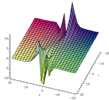
(26)In Figure 1 we can see the 3-D result of first extended model of shallow water wave equation by VIM.
4. VIM Implement for Second Extended
Model of Shallow Water Wave Equation
At last we consider the application of VIM for second extended model of shallow water wave equation with the initial condition given by Equation (19).
Its correction variational functional in x and t can be expressed, respectively, as follows:
3
1 0 2
0 3 3 , , , , , , ,
3 , 3 d
, , ,
6 , d
t n n
n n
x
n n n
n
n n n
n
u x u x u x t u x t
x u x u x u u x
x
u x u x u x
u x
x x x
(27)where is general Lagrangian multiplier.
After some calculations, we obtain the following sta-tionary conditions:
0 (28)
[image:3.595.305.531.76.284.2]1 t
Figure 1. For the first extended model of shallow water wave equation with the first initial condition (24) of Equa-tion (14), when c = 2.
Thus we have:
t 1, (30) As a result, we obtain the following iteration formula:
1 3 2 0 0 3 3 , , , , 3 , , , , 3 d , ,6 , d
n n
t n n n
n
x
n n n
n n
n
u x t u x t
u x u x u x
u x x
u x u u x
x x
u x u x
u x x x ,
(31)We start with the initial approximation of u x
, 0 given by Equation (19). Using the above iteration for- mula (31), we can directly obtain the other components as follows:
2 0
1 1
1 sec h
2 1 , 2 2 c c x c u x t
c
(32)
1 2 3 1 , 1 1 cosh 1 2 11 1 1 1
( 1) cosh cosh
2 2 1 2
1 1 1
2 sinh ,
2 1 1
u x t
c x c c
c c
c c x x
c c
c c x t c c c 1
1 (33)
0
M. SAFARI ET AL. 238
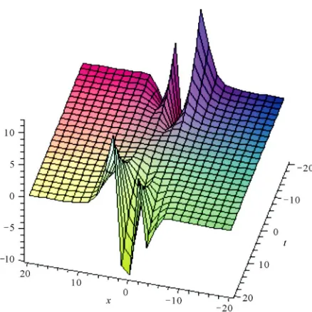
Figure 2. For the second extended model of shallow water wave equation with the first initial condition (32) of Equa-tion (16), when c = 2.
2 1
3
1 1 1
1 2
0
1 1 1
0 3
1 1
1 3
, ,
, ,
3 ,
, , ,
3 d
, ,
6 , d
t
x
u x t u x t
u x u x u x
u x x
u x u u x
x x
u x u x
u x
x x
,
(34)In Figure 2 we can see the 3-D result of second
ex-tended model of shallow water wave equation by VIM.
5. Acknowledgements
In this paper, He’s variational iteration method has been successfully applied to find the solution of two extended model equations for shallow water. The obtained results were showed graphically it is proved that He’s varia- tional iteration method is a powerful method for solving these equations. In our work; we used the Maple Package to calculate the functions obtained from the He’s varia- tional iteration method.
6. References
[1] P. A. Clarkson and E. L. Mansfield, “On a Shallow Water Wave Equation,” Nonlinearity, Vol. 7, No. 3, 1994, pp. 975-1000. doi:10.1088/0951-7715/7/3/012
[2] M. J. Ablowitz, D. J. Kaup, A. C. Newell and H. Segur, “The Inverse Scattering Transform-Fourier Analysis for
Nonlinear Problems,” Studies in Applied Mathematics, Vol. 53, 1974, pp.249-315.
[3] R. Hirota and J. Satsuma,” Soliton Solutions of Model Equations for Shallow Water Waves,” Journal of the
Physical Society of Japan, Vol. 40, No. 2, 1976, pp. 611- 612. doi:10.1143/JPSJ.40.611
[4] J. H. He, “Some Asymptotic Methods for Strongly Non- linear Equations,” International Journal of Modern Phy-
sics B, Vol. 20, No. 10, 2006, pp. 1141-1199. doi:10.1142/S0217979206033796
[5] J. H. He, “Approximate Analytical Solution for Seepage Flow with Fractional Derivatives in Porous Media,” Com-
puter Methods in Applied Mechanics and Engineering, Vol. 167, No. 1-2, 1998, pp. 57-68.
doi:10.1016/S0045-7825(98)00108-X
[6] J. H. He, “Variational Iteration Method for Autonomous Ordinary Differential Systems,” Applied Mathematics and
Computation, Vol. 114, No. 2-3, 2000, pp. 115-123. doi:10.1016/S0096-3003(99)00104-6
[7] J. H. He and X. H. Wu, “Construction of Solitary Solu- tion and Compacton-Like Solution by Variational Itera- tion Method,” Chaos Solitons & Fractals, Vol. 29, No. 1, 2006, pp. 108-113. doi:10.1016/j.chaos.2005.10.100
[8] J. H. He, “A New Approach to Nonlinear Partial Differ-ential Equations”, Communications in Nonlinear Science
and Numerical Simulation, Vol. 2, No. 4, 1997, pp. 203- 205. doi:10.1016/S1007-5704(97)90007-1
[9] J. H. He, “Variational Iteration Method—A Kind of Non- linear Analytical Technique: Some Examples,” Interna-
tional Journal of Nonlinear Mechanics, Vol. 34, No. 4, 1999, pp. 699-708. doi:10.1016/S0020-7462(98)00048-1
[10] J. H. He, “A Generalized Variational Principle in Micro- morphic Thermoelasticity,” Mechanics Research Commu-
nications, Vol. 32, No. 1, 2005, pp. 93-98. doi:10.1016/j.mechrescom.2004.06.006
[11] D. D. Ganji, M. Jannatabadi and E. Mohseni, “Applica- tion of He’s Variational Iteration Method to Nonlinear Jaulent-Miodek Equations and Comparing It with ADM,”
Journal of Computional and Applied Mathematics, Vol. 207, No. 1, 2007, pp. 35-45.
[12] D. D. Ganji, E. M. M. Sadeghi and M. Safari, “Appli- cation of He’s Variational Iteration Method and Ado- mian’s Decomposition Method Method to Prochhammer Chree Equation,” International Journal of Modern Phy-
sics B, Vol. 23, No. 3, 2009, pp. 435-446. doi:10.1142/S0217979209049656
[13] M. Safari, D. D. Ganji and M. Moslemi, “Application of He’s Variational Iteration Method and Adomian’s De-composition Method to the Fractional KdV-Burgers- Kuramoto Equation,” Computers and Mathematics with
Applications, Vol. 58, No. 11-12, 2009, pp. 2091-2097. [14] M. Safari, D. D. Ganji and E. M. M. Sadeghi, “Appli-
cation of He’s Homotopy Perturbation and He’s Varia- tional Iteration Methods for Solution of Benney-Lin Equation,” International Journal of Computer Mathema-
[15] D. D. Ganji, M. Safari and R. Ghayor, “Application of He’s Variational Iteration Method and Adomian’s De- composition Method to Sawada-Kotera-Ito Seventh-Order
Equation”, Numerical Methods for Partial Differential