Automatic Abnormal Electroencephalograms Detection of Preterm Infants

(1)

ISSN Online: 2327-7203 ISSN Print: 2327-7211

DOI: 10.4236/jdaip.2018.64009 Nov. 12, 2018 141 Journal of Data Analysis and Information Processing

Automatic Abnormal Electroencephalograms

Detection of Preterm Infants

Daniel Schang

1

, Pierre Chauvet

2

, Sylvie Nguyen The Tich

3

, Bassam Daya

4

, Nisrine Jrad

2

,

Marc Gibaud

5

1_{ESEO Tech, Angers, France} 2_{UCO-LARIS-UBL, Angers, France}

3_{CHRU de Lille, Hopital Albert Calmette, Lille, France} 4_{Institute of Technology, Lebanese University, Saida, Lebanon} 5_{CHU-LARIS-UBL, Angers, France}

Abstract

Many preterm infants suffer from neural disorders caused by early birth complications. The detection of children with neurological risk is an impor-tant challenge. The electroencephalogram is an imporimpor-tant technique for es-tablishing long-term neurological prognosis. Within this scope, the goal of this study is to propose an automatic detection of abnormal preterm babies’ electroencephalograms (EEG). A corpus of 316 neonatal EEG recordings of 100 infants born after less than 35 weeks of gestation were preprocessed and a time series of standard deviation was computed. This time series was thre-sholded to detect Inter Burst Intervals (IBI). Temporal features were ex-tracted from bursts and IBI. Feature selection was carried out with classifica-tion in one step so as to select the best combinaclassifica-tion of features in terms of classification performance. Two classifiers were tested: Multiple Linear Re-gressions and Support Vector Machines (SVM). Performance was computed using cross validations. Methods were validated on a corpus of 100 infants with no serious brain damage. The Multiple Linear Regression method shows the best results with a sensitivity of 86.11% ± 10.01%, a specificity of 77.44% ± 7.62% and an AUC (Area under the ROC curves) of 0.82 ± 0.04. An accurate detection of abnormal EEG for preterm infants is feasible. This study is a first step towards an automatic analysis of the premature brain, making it possible to lighten the physician’s workload in the future.

Keywords

Automatic EEG Analysis, Machine Learning, Multiple Linear Regressions,

How to cite this paper: Schang, D., Chau-vet, P., Tich, S.N.T., Daya, B., Jrad, N. and Gibaud, M. (2018) Automatic Abnormal Electroencephalograms Detection of Pre-term Infants. Journal of Data Analysis and Information Processing, 6, 141-155. https://doi.org/10.4236/jdaip.2018.64009 Received: October 5, 2018

Accepted: November 9, 2018 Published: November 12, 2018

http://creativecommons.org/licenses/by/4.0/

(2)

DOI: 10.4236/jdaip.2018.64009 142 Journal of Data Analysis and Information Processing

Preterm Infants, Support Vector Machines

1. Introduction

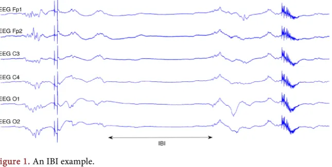
About 15 million newborns are born prematurely every year in the world [1]. Unfortunately, many of the surviving babies suffer from lifetime disabilities such as visual and auditory problems, attention difficulties, and learning problems, etc. To avoid these pathologies, it is essential to diagnose, prognose, and treat preterm born babies as early and as accurately as possible [2] [3]. Usually, preterm babies receive a sustained attention provided by neonatal intensive care units through brain magnetic resonance images, ultrasound assessment or EEG. Non-invasive EEG signals record electrical activity of the brain through electrodes placed along the scalp. EEG signals measure voltage fluctuations resulting from ionic current flows within the neurons of the brain. This technique gives precious information on the ongoing neurological status of a patient and remains a major diagnostic tool for neurology in many situations such as epilepsy, sleep disorders and coma [4]-[10]. As shown in Figure 1, for preterm infants, EEG is physiologically formed by an alternation of bursts of activity and periods of quiescence, called interburst intervals (IBI). The duration and the proportion of IBI vary according to the sleep stages; they are more prolonged in calm sleep. According to the term of birth, they are more prolonged for more premature babies.

[image:2.595.212.535.560.723.2]

During the past four decades, several studies exploited preterm babies EEG to study neural disorders. Intensive studies focused on the neurological outcome of neonatal EEG [11]-[17]. Authors of [18] and [17] defined poor outcome as death or survival with neurodevelopment impairment and good outcome as survival without impairment. In [18], the authors evaluate the correlation between the characteristics of the amplitude-integrated EEG (aEEG), the cerebral ultrasound assessment and the further neurodevelopmental outcome at 3 years of age in premature infants born after less than 30 weeks of gestation. They conclude that

(3)

aEEG is an accurate method for establishing long-term neurological prognosis with sensitivities and specificities comparable to cerebral ultrasound assessment. In [17], the authors note a significant correlation between the long-term neurological prognosis of preterm infants and the IBI value measured from the aEEG in the first 3 days. More recently [19], a meta-analysis confirms the value of EEG in establishing long-term prognosis in premature infants. In everyday clinical practice, the EEG analysis is still done by visual analysis which leads to several difficulties. First, physicians used to analyse EEGs of very preterm infants are rare, often causing delays in the interpretation of EEG tracings, as well as issues related to subjectivity in the analysis. On the other hand, in small hospitals, expertise is often not available. Therefore, within the current trend towards developing automatic diagnostic aid methods, the goal of this paper is to propose a method for automatically predicting the physician’s EEG analysis (abnormal EEG versus normal EEG).

Several studies tried to automatize bursts detection and seizures occurrences (uncontrolled electrical activity in the brain, producing physical convulsions, minor physical signs, thought disturbance, or a combination of those symptoms). For instance, authors of [20], suggested a method for discriminating between seizure and non-seizure EEG epochs of full-term infants. They extracted features, in the time domain, frequency domain and information theory domains from 17 full-term newborns. Features were then classified using a Support Vector Machine (SVM) into seizure and non-seizure EEG. It is noteworthy that EEG characteristics vary a lot between preterm babies and full term babies [21]and are therefore very different from adults EEG. Few studies tackle the problem of identifying abnormal EEG of preterm infants. Within the scope of automatic EEG analysis for premature newborns, we can put forward the work presented by [3]. The authors proposed a method for automated burst detection in the EEG. The detection is based on line length; this length is the running sum of the absolute differences between all consecutive samples into a predefined window [22]. The corpus consisted of 10 preterm infants with a gestational age of less than 34 weeks. It is worth noting that in these approaches [3][17][18][20] the retrospective investigation was done without prospective investigation, which may induce inherent biases.

(4)

systematically used. Finally the standard deviation of the sensitivity is very high, this could conduce to over fitting of the predictive model that has been retained.

The method outlined in this paper works in four steps. First, a preprocessing stage: EEG was filtered, using a band-stop IIR filter and smoothed using a moving average window. Secondly, IBI were detected by thresholding standard deviation of preprocessed EEG. Thirdly, temporal features were extracted from IBI and bursts. Finally, feature selection was incorporated in the classification step so as to select relevant features that maximize classification performance. Two classifiers were tested: Support Vector Machines (SVM) and Multiple Linear Regressions with all combinations of features. Performance measures were evaluated using areas under the ROC curves (AUC, [24] [25]). The proposed method was validated on a cohort of 100 preterm babies with no severe brain injuries.

The paper is outlined as follows: Section 2 describes the collected database. Section 3 accounts for the method. While Section 4 describes the results, Section 5 provides a discussion. Finally a conclusion is drawn and some future works are suggested.

2. Materials

EEG signals from 100 preterm infants were collected in the Hospital of Angers, France, at the neonatal intensive care unit of the neuropediatric department. This monitoring was part of the usual clinical follow up of premature infants. All legal representatives of the babies gave informed consent for participation in research studies. EEG were recorded at sampling rate of 256 Hz. The recording system (Alliance from Nicolet Biomedical) was used with 8 to 11 adapted scalp electrodes according to the head size. Therefore, each EEG was composed of 11 channels. Electrodes were placed according to the international 10 to 20 system (Figure 2). In the acquisition procedure, we did not use any hard filters besides the internal filters of the EEG device; we used only a software high-pass filter with 0.1 Hz as a cut-off frequency, which is used to remove the offset of the baseline.

Thus, 416 neonatal EEG recordings lasting from 30 to 45 minutes were performed between January 1, 2003 and December 31, 2004. All 100 infants had less than 35 weeks of gestation. Each baby had between 1 to 7 recordings.

(5)

[image:5.595.291.457.73.262.2]

Figure 2. Names and positions of electrodes from [26].

30.01 ± 2.19 weeks of gestation). An example of abnormal EEG is illustrated in Figure 1 showing the phenomenon of IBI.

3. Methods

3.1. Problem Statement

Let s t

( )

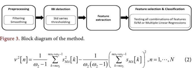
denoting the EEG signal of N samples recorded in a given channel, in which abnormal EEG have to be detected. The EEG signal essentially contains background activity where bursts appear together with abnormal activities (IBI with discontinuity, seizures, rolandic sharp waves, etc.). The problem we address in this paper consists first in detecting the IBI and secondly classifying EEG into normal or abnormal. Automatic detection of abnormal EEG works in four steps summarized in Figure 3: preprocessing, IBI detection, feature extraction, feature selection and classification. In this section, each of these steps will be detailed.

3.2. Preprocessing

For each channel, raw EEG signal s t

( )

has been band-stop filtered at 50 Hz with a notch second order Butterworth IIR filter. Thus, we obtained a filtered signal sBP

( )

t where the power supply frequency of 50 Hz was removed. Then,

( )

BP

s t has been smoothed by calculating the moving average over a window of width ω1:

[ ]

1

[ ]

1

2

2 1

1 n _, _{1, ,}

MA BP

k n

s n ω s k n N

ω

+

= −

=

∑

=  (1)

3.3. Inter Burst Intervals Detection

For detecting IBI, the standard deviation of signal sMA

( )

t has been computed and thresholded as in the work of [27]. Standard deviation has been computed on sliding windows of size ω2, with an overlap of ω3 samples (ω3<ω2) as in

(6)

[image:6.595.207.543.65.183.2]

Figure 3. Block diagram of the method.

[ ]

3 2

[ ]

₍

₎

3 2

[ ]

3 3

2

1 1

2 2

2 2 2

1 1 _, _{1, ,}

1 1

n n

MA MA

k n k n

n ω ω s k ω ω s k n N

ω ω

ν

ω

ω ω

+ − + −

= =

 

= ₋ −   =

−  

∑

 (2)

Successive standard deviation segments with values less than a threshold VT

(in μV) and longer than 1 s have been detected and delimited by an onset and an offset boundary limit markers. Consecutive detections less than 0.5 s apart have been grouped together and considered as the same IBI. Finally, only IBI present across all 11 EEG channels and longer than 1 s have been kept. Noteworthily, it is highly crucial to set the threshold VT so as to get the best performance.

Hence, 100 different values of threshold VT, selected from 1 to 100 μV with a

step of 1, have been tested.

3.4. Feature Extraction

For each EEG of 11 channels, a vector of 13 features has been extracted as following:

1) the number of IBI, called nb_IBI,

2) the total duration of IBI, which is defined as the sum of all IBI durations, called tot_IBI (seconds),

3) the percentage of IBI in the EEG, called _

( )

% _ _ tot IBI P IBI

EEG duration

= _,

4) the duration of the longest IBI, called Max_IBI (seconds), 5) the maximum of IBI percentage in the EEG, called

( )

_

_ _ %

_ Max IBI P Max IBI

EEG duration

= _,

6) the mean duration of IBI which is defined as the sum of the IBI durations divided by the number of IBI, called Mean_IBI (seconds),

7) the number of bursts, called nb_B,

8) the total duration of the bursts that are calculated as the sum of all bursts durations, called tot_B (seconds),

9) the percentage of bursts in the EEG, called _ %

( )

_ _ tot B P B

EEG duration

= _,

10) the duration of the longest burst, called Max_B (seconds), 11) the maximum of bursts percentage in the EEG, called

( )

_

_ _ %

_ Max B P Max B

EEG duration

= _,

12) the mean duration of the bursts was calculated as the sum of the bursts durations divided by the number of bursts, called Mean_B (seconds),

13) the gestational age of the infant at the time of the EEG examination, called

(7)

3.5. Feature Selection and Classification

The extracted features and the gestational age form a set of vectors

13_, _{1, ,}

m

x ∈_ m= _ M _with_M_{the total number of EEG. The entire data set is}

written as

{

(

x y1, 1

)

, ,

(

x ym, m

)

, ,

(

x yM, M

)

}

with class labels ym∈ + −

{

1, 1

}

for Abnormal and Normal EEG respectively. The task hereafter consists of selecting relevant features and discriminating EEG into Abnormal or Normal. Two classifiers were compared: Support Vector Machines (SVM) and Multiple Linear Regressions. In the following, feature selection is explained in the context of both classification methods.

3.5.1. Support Vector Machines

Feature extraction was done along with SVM classification [28]-[36]. We will now very briefly describe the principles underlying the SVM principles.

Technically, SVM separate the data set

(

)

(

)

(

)

{

x y1, 1 , , x ym, m , , , x yM M

}

∈d× −

{

1,1

}

by a hyperplane with the

largest possible margin and the minimal number of misclassified data. This hyperplane is defined by a weight vector _w_∈_d_,_d_{being the dimension of}

feature vectors, and an offset b∈__{as following:}

(

)

: d { 1,1}

m m

H

x sign w x b

→ −

⋅ +





(3)

This hyperplane is calculated by solving an optimization problem under constraints:

(

)

2 1 1 2

subject to : 1 0,

M m m

m m m m

w C

w x b y m

ξ ξ ξ =  ₊  

 _⋅ ₊ _{≥ −} _{> ∀}



∑

₍₄₎

2 1

2 w is the maximal margin hyperplane, C is the regularization parameter

and ξm are the nonnegative slack variables [34] measuring errors.

By setting to zero the derivatives of the partial associated Lagrangian according to the primal variables w b, and ξm, the optimization problem of

the dual formulation can be written as:

1 , 1

1

1 _,

2

subject to : 0 and 0

M M

m m p m p m p

m m p

M

m m m

m

y y x x y

α α α

α α = = =  ₋    _≤ ₌ 

∑

(5)

The linear SVM is extended to a non-linear classifier by mapping data into a higher dimension space using a mapping function Φ_{, then the optimization}

problem becomes as follows:

(

)

1 , 1

1

1 _,

2

subject to : 0 and 0

M M

m m p m p m p

m m p

M

m m m

m

y y K x x y

α α α

α α = = =  ₋    _≤ ₌ 

∑

(8)

where K designs the kernel function. The hyperplane solution has the final following formulation:

( )

(

)

1 ,

M

m m m

m

h x α y K x x b

=

∑

+ ₍₇₎

Several kernels were tested, namely Radial basis function kernels (RBF), polynomial kernels and linear kernels. As for the dimension d of input data, all combinations of the 13 features were tested for each kernel. This results in testing ₂13_{− =}_{1 8191}_{combinations for each kernel and for each of the 100}

threshold values aforementioned in 3.

For the implementations, we used Matlab© (The Mathworks Inc., South Natic, MA, USA) and the LS-SVM 1.8 toolbox that provides a complete implementation of SVM [37].

3.5.2. Multiple Linear Regressions

Multiple linear regression is a generalization of the simple linear regression method [38]. This method attempts to model the relationship between a response variable and explanatory variables. Suppose we have n observations and p explanatory variables, with Yi the n variables to be predicted and

1, , , 1, ,

i ip

X  X i=  p the explanatory variables, we have the following equation:

0 1 1 2 2 , 1, ,

i i i p ip i

Y a a X= + +a X + +_ a X + i= _ n (8)

where the coefficients a a0, , ,1 ap are the parameters to be estimated and i

are the errors of the model that expresses the missing informations.

Like for SVM, all combinations of the 13 explanatory variables for each threshold were tested.

3.6. Performance Evaluation

To evaluate the accuracy of the predictions, two parameters were used: the sensitivity and the specificity. The percentages of sensitivity and specificity were computed as follows:

 sensitivity 100= ×TP TP FN

(

+

)

_,

 specificity 100= ×TN TN FP

(

+

)

_with:

- TP: number of true positives, TN: number of true negatives, - FN: number of false negatives, FP: number of false positives.

The use of sensitivities and specificities is based on a precondition: the distribution of “normal” and “abnormal” EEG must be significantly balanced. We reached a prevalence of 11.23%, so this condition of data balance was not met by the corpus of EEG. Therefore, ROC curves were used [24]: this curve-based method is independent of class distribution and independent of misclassification data proportion. By plotting sensitivity versus 1—specificity for different cutoff values, the ROC curves were built. The area under the curve reflects the accuracy of the test: a high area gives a high test accuracy [24].

(9)

we used a K-fold cross-validation [39] (K equal to 5). So, the data set is randomly divided into K equal subsets (called folds). The classifier is trained on

1

K− _{folds; the validation performances are then measured on the remaining}

fold that was not used during the training phase. The process is repeated K times by using the remaining fold to estimate the validation errors: thus, the performance of the classifier is obtained by averaging the K AUC. The latter area gives us an overall accuracy for each ROC curve; therefore to reach the best threshold for each curve, the best sensitivity and the best specificity have been computed by minimizing the quantity:

2 2

sensitivity specificity

1 1

100 100

 ₋  _{+ −} 

   

    (9)

The 5 subsets were built randomly; just keeping an equivalent number of children in each subset: due to the number of 42 abnormal EEG (indivisible by 5), we had 3 sets of 8 abnormal EEG and 2 sets with 9 abnormal EEG.

During the 5 cross validations, 3 kernels (linear, polynomial and gaussian radial basis) were tested. For the polynomial kernel, the degree varied from 3 to 5. The gaussian radial basis worked with σ∈

[

0.1;2.0

]

_{. The optimal SVM} kernels (linear, polynomial and gaussian radial basis) that gave the highest mean value of the K AUC were retained.

4. Results

Table 1 shows performance of all classifiers as a mean ± standard deviation of sensitivity, specificity and AUC. It is clear that the Multiple Linear Regression method achieved the best performance with a mean sensitivity of

86.11% 10.01%± _{, a mean specificity of}77.44% 7.62%± _{and a mean AUC of} 0.82 0.04± _{. The selected threshold}V_T was equal to 32 μV. The best combination of features was obtained with 11 features: Age_EEG, nb_IBI,

tot_IBI, P_IBI, Max_IBI, P_Max_IBI, Mean_IBI, nb_B, P_B, P_Max_B and

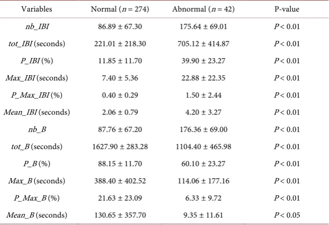
Mean_B (see Table 2 for the descriptive statistics of all extracted features for the best threshold VT equal to 32 μV).

For linear SVM, the threshold was 35 μV and the selected features were:

nb_IBI, P_IBI, P_Max_IBI Mean_IBI, nb_B, P_Max_B. SVM with polynomial kernels reached the optimal performance with a threshold equal to 32 μV using

Age_EEG, tot_IBI, P_IBI, Max_IBI, tot_B, P_B, Max_B, P_Max_B, Mean_B. Finally, the gaussian SVM used only 3 features Age_EEG, Mean_IBI, nb_B, with a threshold equal to 25 μV.

The final detector was trained on all the corpus with the Multiple Linear Regression method on the 11 features Age_EEG, nb_IBI, tot_IBI, P_IBI,

Max_IBI, P_Max_IBI, Mean_IBI, nb_B, P_B, P_Max_B and Mean_B. With the

prediction set to +1 (Abnormal) and −1 (Normal), we obtained the Equation (10) which is detailed in the following.

1 2 3 4 5 6

7 8 9 10 11

0.1936 0.1929 0.1893 0.1246 0.0623 0.0286 0.0104 0.001 0.0007 0.0005 0.0002

P x x x x x x

x x x x x

= − − + + + −

(10)

[image:10.595.206.541.90.174.2]

Table 1. 5-cross validation results.

Method Sensitivity (%) Specificity (%) AUC

SVM linear kernels 48.37 ± 13.97 98.19 ± 2.23 0.73 ± 0.06

SVM polynomial kernels 53.17 ± 11.20 97.08 ± 1.63 0.75 ± 0.06

SVM RBF kernels 53.17 ± 11.20 98.55 ± 1.52 0.76 ± 0.05

Multiple linear regression 86.11 ± 10.01 77.44 ± 7.62 0.82 ± 0.04

Table 2. Extracted features for a threshold equal to 32 μV.

Variables Normal (n = 274) Abnormal (n = 42) P-value

nb_IBI 86.89 ± 67.30 175.64 ± 69.01 P < 0.01

tot_IBI (seconds) 221.01 ± 218.30 705.12 ± 414.87 P < 0.01

P_IBI (%) 11.85 ± 11.70 39.90 ± 23.27 P < 0.01

Max_IBI (seconds) 7.40 ± 5.36 22.88 ± 22.35 P < 0.01

P_Max_IBI (%) 0.40 ± 0.29 1.50 ± 2.44 P < 0.01

Mean_IBI (seconds) 2.06 ± 0.79 4.20 ± 3.27 P < 0.01

nb_B 87.76 ± 67.20 176.36 ± 69.00 P < 0.01

tot_B (seconds) 1627.90 ± 283.28 1104.40 ± 465.98 P < 0.01

P_B (%) 88.15 ± 11.70 60.10 ± 23.27 P < 0.01

Max_B (seconds) 388.40 ± 402.52 114.06 ± 177.16 P < 0.01

P_Max_B (%) 21.63 ± 23.09 6.33 ± 9.72 P < 0.01

Mean_B (seconds) 130.65 ± 357.70 9.35 ± 11.61 P < 0.05

where variable P represents the variable prediction, variable x1 represents

Mean_IBI, variable x2 represents nb_IBI,..., variable x11 represents Mean_B (all variables are shown in Table 3). Therefore, Equation (10) shows the weight (impact) of features on the prediction and their positive or negative correlations with prognosis. The weight associated to each feature and their cumulative values are shown in Table 3.

All calculations were performed on computers equipped with Intel Core i5-3470 CPU at 3.20 GHz, 8 Go of RAM under Linux Ubuntu. We used 10 computers simultaneously: for the 100 thresholds, the linear SVM kernels took 9 days and 14 hours. While the polynomials SVM kernels took 65 days and 8 hours, only 10 days and 2 hours were necessary for the RBF SVM kernels. Finally, the Multiple Linear Regressions took only 59 minutes on one computer.

5. Discussion

Experimental results show that a Multiple Linear Regression estimated on 11 features (Age_EEG, nb_IBI, tot_IBI, P_IBI, Max_IBI, P_Max_IBI, Mean_IBI,

[image:10.595.212.539.209.432.2]

(11)

[image:11.595.207.540.88.294.2]

Table 3. The impact and cumulative impact of each variable.

Variables Weight (in %) Cumulative weight (in %)

Mean_IBI 24.08 24.08

nb_IBI 23.99 48.06

nb_B 23.54 71.60

P_Max_IBI 15.50 87.10

Age_EEG 7.75 94.85

P_B 3.56 98.41

P_IBI 1.29 99.70

Max_IBI 0.12 99.82

tot_IBI 0.09 99.91

P_Max_B 0.06 99.97

Mean_B 0.02 100.00

the automatic detection considers that an EEG is abnormal, it must be interpreted also by the neurologist before undergoing more medical examinations such as an MRI (Magnetic Resonance Imaging). Finally, due to the high sensitivity of our test, an EEG classified as normal does not need to be interpreted urgently by the doctor.

A main advantage of the proposed method is that threshold and feature selection are tuned so as to maximize classification performance. There are of course several ways to select threshold and features [40] [41][42][43][44]; but they are not optimal from a classification point of view.

When comparing SVM to Multiple Linear Regressions, we can see that computational time of linear SVM is 1.32 × 106_{times slower, RBF SVM is 1.46 ×} 106_{times slower and polynomial SVM is 9.52 × 10}6_{times slower than that of} regressions. Besides, Multiple Linear Regressions performance are higher than SVM ones. However, SVM results are promising, namely those obtained with RBF SVM kernels where only 3 variables were selected (Age_EEG, Mean_IBI,

nb_B). This sparsity in feature selection could enhance the robustness of our learning machines [45] [46]. It is to note that the Multiple Linear Regression method captures almost 95% of the prediction process with 5 variables (Mean_IBI, nb_IBI, nb_B, P_Max_IBI, Age_EEG), as can be seen in the cumulative expressive power (Table 3).

(12)

for this is essentially because it would have taken too long to test all the combinations with neural networks.

6. Conclusions

This study suggests an automated method to detect abnormal Electroencepha- lograms (EEG) of preterm infants. The novelty of this paper lies in the combination of these three facts: firstly we work on preterm infants; secondly we propose to automatize the current diagnosis and not to automatize a long term neurological outcome and thirdly this automated prediction is evaluated in a prospective group and not only in a retrospective group. The method consists of detecting Inter Burst Intervals, extracting features from EEG, selecting relevant features and classifying them into normal or abnormal EEG. Thus, gestational age and 10 features (N_IBI, TOT_IBI, P_IBI, MAX_IBI, P_MAX_IBI, MEAN_IBI, N_B,

P_B, P_MAX_B, MEAN_B) extracted from the EEG and introduced in a Multiple Linear Regression model, could reliably predict an abnormal finding with a sensitivity of 86.11% ± 10.01%, a specificity of 77.44% ± 7.62% and an AUC of 0.82 ± 0.04.

These results are very promising and encourage further research that could enhance detection of abnormal EEG, namely considering more features, like frequency and information theory features for instance. Finally, testing combination of several classifiers could be a promising path of research too.

Acknowledgements

This research was paid by no grant. Sincere thanks to J.F. Gelfi and R. Woodward for their help in the improvement of the quality of this paper.

Conflicts of Interest

The authors declare no conflicts of interest.

References

[1] Blencowe, H., Cousens, S., Oestergaard, M.Z., Chou, D., Moller, A.B., Narwal, R., Adler A., Vera Garcia, C., Rohde, S., Say, L. and Lawn, J.E. (2012) National, Region-al, and Worldwide Estimates of Preterm Birth Rates in the Year 2010 with Time Trends since 1990 for Selected Countries: A Systematic Analysis and Implications. The Lancet, 379, 2162-2172.https://doi.org/10.1016/S0140-6736(12)60820-4 [2] Deburchgraeve, W., Cherian, P.J., De Vos, M., Swarte, R.M., Blok, J.H., Visser, G.H,

Govaert, P. and Van Huffel, S. (2008) Automated Neonatal Seizure Detection Mi-micking a Human Observer Reading EEG. Clinical Neurophysiology, 119, 2447-2454. https://doi.org/10.1016/j.clinph.2008.07.281

[3] Koolen, N., Jansen, K., Vervisch, J., Matic, V., De Vos, M., Naulaers, G. and Van Huffel, S. (2014) Line Length as a Robust Method to Detect High-Activity Envents: Automated Burst Detection in Premature EEG Recordings. Clinical Neurophysiol-ogy, 125, 1985-1994. https://doi.org/10.1016/j.clinph.2014.02.015

(13)

[5] Lima, C.A.M. and Coelho, A.L.V. (2011) Kernel Machines for Epilepsy Diagnosis via EEG Signal Classification: A Comparative Study. Artificial Intelligence in Medi-cine, 53, 83-95.

[6] Tang, Y. and Durand, D.M. (2012) A Tunable Support Vector Machine Assembly Classifier for Epileptic Seizure Detection. Expert Systems with Applications, 39, 3925-3938. https://doi.org/10.1016/j.eswa.2011.08.088

[7] Musselman, M. and Djurdjanovic, D. (2012) Time Frequency Distributions in the Classification of Epilepsy from EEG Signals. Expert Systems with Applications, 39, 11413-11422. https://doi.org/10.1016/j.eswa.2012.04.023

[8] Boylan, G.B., Stevenson, N.J. and Vanhatalo, S. (2013) Monitoring Neonatal Sei-zures. Seminars in Fetal and Neonatal Medicine, 18, 202-208.

https://doi.org/10.1016/j.siny.2013.04.004

[9] Lee, S.H., Lim, J.S., Kim, J.K., Yang, J. and Lee, Y. (2014) Classification of Normal and Epileptic Seizure EEG Signals Using Wavelet Transform, Phase-Space Recon-struction, and Euclidean Distance. Computer Methods and Programs in Biomedi-cine, 116, 10-25. https://doi.org/10.1016/j.cmpb.2014.04.012

[10] Chen, G. (2014) Automatic EEG Seizure Detection Using Dual-Tree Complex Wavelet-Fourier Features. Expert Systems with Applications, 41, 2391-2394. https://doi.org/10.1016/j.eswa.2013.09.037

[11] Rose, A.L. and Lombroso, C.T. (1970) A Study of Clinical, Pathological, and Elec-troencephalographic Features in 137 Full-Term Babies with a long-Term Fol-low-Up. Pediatrics, 45, 404-425.

[12] Tharp, B.R, Cukier, F. and Monod, N. (1981) The Prognostic Value of the Elec-troencephalogram in Premature Infants. Electroencephalography and Clinical Neurophysiology, 51, 219-236. https://doi.org/10.1016/0013-4694(81)90136-X [13] Holmes, C.L. and Lombroso, C.T. (1993) Prognostic Value of Background Patterns

in the Neonatal EEG. Clinical Neurophysiology, 10, 323-352. https://doi.org/10.1097/00004691-199307000-00008

[14] Menache, C.C., Bourgeois, B.F. and Volpe, J.J. (2002) Prognostic Value of Neonatal Discontinuous EEG. Pediatric Neurology, 27, 93-101.

https://doi.org/10.1016/S0887-8994(02)00396-X

[15] Cilio, M.R. (2009) EEG and the Newborn. Pediatric Neurology, 7, 25-43.

[16] Bowen, J.R., Paradisis, M. and Shah, D. (2010) Decreased aEEG Continuity and Baseline Variability in the First 48 Hours of Life Associated with Poor Short-Term Outcome in Neonates born before 29 Weeks Gestation. Pediatric Research, 67, 538-544.https://doi.org/10.1203/PDR.0b013e3181d4ecda

[17] Wikstrom, S., Pupp, I.H., Rosen, I., Norman, E., Fellman, V., Ley, D. and Hellstrom-Westas, L. (2012) Early Single-Channel aEEG/EEG Predicts Outcome in Very Preterm Infants. Acta Paediatrica, 101, 719-726.

https://doi.org/10.1111/j.1651-2227.2012.02677.x

[18] Klebermass, K., Olischar, M., Waldhoer, T., Fuiko, R. and Weninger, A. (2011) Amplitude-Integrated Electroencephalography Pattern Predicts Further Outcome in Preterm Infants. Pediatric Research, 70, 102-108.

https://doi.org/10.1203/PDR.0b013e31821ba200

[19] Fogtmann, E.P., Plomgaard, A.M., Greisen, G. and Gluud, C. (2017) Prognostic Accuracy of Electroencephalograms in Preterm Infants: A Systematic Review. Pe-diatrics, 139, 1-14.https://doi.org/10.1542/peds.2016-1951

(14)

EEG-Based Neonatal Seizure Detection with Support Vector Machines. Clinical Neurophysiology, 122, 464-473.https://doi.org/10.1016/j.clinph.2010.06.034 [21] Joseph, J.P., Lesevre, N. and Dreyfus-Brisac, C. (1976) Spatio-Temporal

Organiza-tion of EEG in Premature Infants and Full-Term New-Borns. Electroencephalogra-phy and Clinical NeuroElectroencephalogra-physiology, 40, 153-168.

https://doi.org/10.1016/0013-4694(76)90160-7

[22] Esteller, R., Echauz, J., Tcheng, T., Litt, B. and Pless, B. (2001) Line Length: An Effi-cient Feature for Seizure Onset Detection. Proceedings of the 23rd Annual Interna-tional Conference on Engineering in Medicine and Biology Society, Instanbul, 1707-1710.

[23] Jrad, N., Schang, D., Chauvet, P., Nguyen the Tich, S., Daya, B. and Gibaud, M. (2017) Automatic Detector of Abnormal EEG for Preterm Infants. Lecture Notes of the Institute for Computer Sciences, Social Informatics and Telecommunications Engineering: 4th International Conference, Vol. 225, 82-87.

[24] Hanley, J.A. and McNeil, B.J. (1982) The Meaning and Use of the Area under a Re-ceiver Operating Characteristic (ROC) Curve. Radiology, 143, 29-36.

https://doi.org/10.1148/radiology.143.1.7063747

[25] Fawcett, T. (2006) An Introduction to ROC Analysis. Pattern Recognition Letters, 27, 861-874.

[26] Shellhaas, R., Chang, T., Tsuchida, T., Scher, M.S., Riviello, J.J., Abend, N.S., Nguyen, S., Wusthoff, C.J. and Clancy, R.R. (2011) The American Clinical Neuro-physiology Society’s Guideline on Continuous Electroencephalography Monitoring in Neonates. Clinical Neurophysiology, 28, 611-617.

https://doi.org/10.1097/WNP.0b013e31823e96d7

[27] Chauvet, P.E., Nguyen The Tich, S., Schang, D. and Clement, A. (2014) Evaluation of Automatic Feature Detection Algorithms in EEG: Application to Interburst In-tervals. Computers in Biology and Medicine, 54, 61-71.

https://doi.org/10.1016/j.compbiomed.2014.08.011

[28] Lukas, L. (2003) Least Squares Support Vector Machines Classification Applied to Brain Tumor Recognition Using Magnetic Resonance Spectroscopy. Ph.D. Thesis, Faculty of Engineering, Leuven.

[29] Lu, C. (2005) Probabilistic Machine Learning Approaches to Medical Classification Problems. Ph.D. Thesis, Faculty of Engineering, Leuven.

[30] Schang, D., Feuilloy, M., Plantier, G., Fortrat, J.O. and Nicolas, P. (2007) Early Pre-diction of Unexplained Syncope by Support Vector Machines. Physiological Mea-surement, 28, 185-197.https://doi.org/10.1088/0967-3334/28/2/007

[31] Yin, Z. and Zhang, J. (2014) Identification of Temporal Variations in Mental Workload Using Locally-Linear-Embedding-Based EEG Feature Reduction and Support-Vector-Machine-Based Clustering and Classification Techniques. Com-puter Methods and Programs in Biomedicine, 115, 119-134.

https://doi.org/10.1016/j.cmpb.2014.04.011

[32] Esfandiari, N., Reza Babavalian, M., Eftekhari Moghadam, A.M. and Kashani Tabar, V. (2014) Knowledge Discovery in Medicine: Current Issue and Future Trend. Ex-pert Systems with Applications, 41, 4434-4463.

https://doi.org/10.1016/j.eswa.2014.01.011

(15)

[34] Vapnik, V. (2000) The Nature of Statistical Learning Theory. Springer, Berlin. https://doi.org/10.1007/978-1-4757-3264-1

[35] Hastie, T., Tibshirani, R. and Friedman, J. (2001) The Elements of Statistical Learn-ing. Springer Series in Statistics. Springer, Berlin.

https://doi.org/10.1007/978-0-387-21606-5

[36] Bishop, C.M. (2006) Pattern Recognition and Machine Learning. Springer, Berlin. [37] Suykens, J.A.K., Van Gestel, T., De Brabanter, J., De Moor, B. and Vandewalle, J.

(2002) Least Squares Support Vector Machines. World Scientific Publishing, Sin-gapore.

[38] Chatterjee, S. and Hadi, A.S. (1986) Influential Observations, High Leverage Points, and Outliers in Linear Regression. Statistical Science, 1, 379-393.

https://doi.org/10.1214/ss/1177013622

[39] Bishop, C.M. (1995) Neural Networks for Pattern Recognition. Oxford University Press, Oxford.

[40] Guyon, I. and Elisseeff, A. (2003) An Introduction to Variable and Feature Selec-tion. Machine Learning Research, 3, 1157-1182.

[41] Stoppiglia, H., Dreyfus, G., Dubois, R. and Oussar, Y. (2003) Ranking a Random Feature for Variable and Feature Selection. Machine Learning Research, 3, 1399-1414.

[42] Yu, L. and Liu, H. (2004) Efficient Feature Selection via Analysis of Relevance and Redundancy. Machine Learning Research, 5, 1205-1224.

[43] Liu, H. and Yu, L. (2005) Toward Integrating Feature Selection Algorithms for Classification and Clustering. IEEE Transactions on Knowledge and Data Engi-neering, 17, 491-502. https://doi.org/10.1109/TKDE.2005.66

[44] Theodoridis, S. and Koutroumbas, K. (2006) Pattern Recognition. Academic Press, Cambridge.

[45] Barron, A. (1993) Universal Approximation Bounds for Superposition of a Sig-moidal Function. IEEE Transactions on Information Theory, 39, 930-945. https://doi.org/10.1109/18.256500