Fuzzy vs. Probabilistic Techniques to Address Uncertainty
for Radial Distribution Load Flow Simulation
Roma Raina1, Mini Thomas2
1
Manipal University, Dubai, UAE
2
Jamia Millia Islamia University, New Delhi, India Email: [email protected]
Received January 8, 2012; revised February 10, 2012; accepted February 22, 2012
ABSTRACT
For Power distribution system the most important task for distribution engineer is to efficiently simulate the system and address the uncertainty using a suitable mathematical method. This paper presents a comparison of two methods used in analyzing uncertainties. The first method is Montecarlo simulation (MCS) that considers input parameters as random variables and second one is fuzzy alpha cut method (FAC) in which uncertain parameters are treated as fuzzy numbers with given membership functions. Both techniques are tested on a typical Load flow solution simulation, where con-nected loads are considered as uncertain. In order to provide a basis for comparison between above two approaches, the shapes of the membership function used in the fuzzy method is taken same as the shape of the probability density func-tion used in the Monte Carlo simulafunc-tions. For more than one uncertain input variable, simulafunc-tion result indicates that MCS method provides better output results compared to FAC, however takes more time due to number of runs. FAC provides an alternate method to MCS when addressing single or limited input variables and is fast.
Keywords: Fuzzy Set; Radial Power Distribution; Montecarlo; Load Flow
1. Introduction
Current time power distribution systems, especially in de-veloping countries, are steadily approaching towards its maximum operating limits and voltage stability is a ma-jor concern. Voltage instability leads to blackouts and makes the system unreliable. It is important to have a reli-able power distribution system, which maintains voltages within the permissible range and ensure a high quality of output.
The voltage instability can be addressed using the various techniques e.g. reconfiguration, addition of capacitor banks etc., however need an efficient simulation of load flow and a mathematical method which address the uncer-tainty efficiently especially the unceruncer-tainty associated with input parameters. Distribution system uncertainties are due to error in measurement of feeder parameters, variation in expected values of the demands with time etc. and are main causes of uncertain simulation outputs.
Uncertainty can be analyzed and addressed using sev-eral techniques. In past, many solution methods have been developed on Load Flow distribution networks using Fuzzy and probabilistic models.
D. M. Falcao describes the conceptual basis and prelimi-nary results of a load estimation based on the application of neural network and fuzzy set techniques [1]. Chi-Wen Liu presents a neurofuzzy network for voltage security
monitoring [2]. I. J. Ramirez-Rosado, Dominguez-Navarro, presents a new possibilistic (fuzzy) model for the mul-tiobjective optimal planning of power distribution net-works [3]. Vikas kumar presents a comparison between probalistic and Fuzzy alpha cut techniques in general [4]. A. J Abebe presents a comparison of two methods (fuzzy alpha cut and Monte Carlo simulation) of analysis of uncertainty arising from uncertain model parameters [5]. However none have been found comparing two methods and addressing importance of each other for radial dis-tribution system calculations.
This paper presents a comparison of “Monte-Carlo simu-lation method (MCS)” a technique based on probability and “Fuzzy alpha cut method (FAC)” a technique based on Fuzzy. The MCS technique treats uncertain parameter as random variable that obeys a given probabilistic distribu-tion and model output is then a random variable. The fuzzy analysis is based on fuzzy logic and fuzzy set theory, which is widely used in representing uncertain knowl-edge. Uncertain model parameters are treated as fuzzy numbers with a membership function.
2. Methodology
2.1. Steps & Input Data
algo-rithm, based on concept described by R. Raina, M Tho-mas, R. Ranjan [6]. The algorithm calculates the total real and reactive system power loss of the radial distribu-tion network. The algorithm considers input parameters as random variables for Monte Carlo simulation and as fuzzy numbers with a given membership function for fuzzy logic.
This simulation is run on a typical 19 bus distribution system from the D. Thukram, H. M W. Banda and J. Jerome [7] shown in Figure 1.
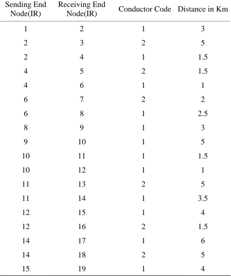
Input connected load data for the feeder are given in Table 1, Conductor data for the feeders are given in Ta-ble 2 and Table 3.
Figure 2 shows the Typical Load Flow calculation chart used for Fuzzy and Monte Carlo simulation. The details of formulas and computing method are in [6].
2.2. Monte-Carlo Simulation Method (MCS)
The MCS principle is described in Figure 3. Uncertain input parameter is considered as a random variable P and numbers of realizations Pi of P are generated and load
flow algorithm is run for each of them producing an out-put Ri. The set of outputs Ri represents the set of
realiza-tions of the random variable R. The statistical properties of R are therefore computed from the realizations Ri.
2.3. Fuzzy Alpha-Cut Method (FAC)
[image:2.595.308.539.460.736.2]This method uses fuzzy set theory to represent uncer-tainty or imprecision in the parameters. Uncertain parame-ters are considered to be fuzzy numbers with some mem-bership functions. In fuzzy logic, it represents the degree of truth as an extension of valuation. Degrees of truth are often confused with probabilities, although they are con-
Figure 1. Shows a practical 19 bus distribution feeder used for the modeling and simulation purpose.
Table 1. Load data.
Phase Load in kVA Node
A B C
2 64 32 64
3 68 32 60
4 25 35 40
5 40 32 28
6 26 19 18
7 60 50 50
8 46 33 21
9 76 92 82
10 21 26 16
11 46 46 68
12 60 50 50
13 27 33 40
14 19 19 25
15 27 30 43
16 48 64 48
17 40 30 30
18 33 33 34
19 54 62 44
Table 2. Conductor data.
Conductor type Resistance PU/Km Reactance PU/Km
1 0.008600 0.003700
2 0.012950 0.003680
Table 3. Conductor code & distances.
Sending End Node(IR)
Receiving End
Node(IR) Conductor Code Distance in Km
1 2 1 3
2 3 2 5
2 4 1 1.5
4 5 2 1.5
4 6 1 1
6 7 2 2
6 8 1 2.5
8 9 1 3
9 10 1 5
10 11 1 1.5
10 12 1 1
11 13 2 5
11 14 1 3.5
12 15 1 4
12 16 2 1.5
14 17 1 6
14 18 2 5
[image:2.595.57.287.514.706.2]Start
Read Fuzzy / Probability interpreted input
IT = 1
I =1
Compute the total power drawn from the bus
Is I<NB? I = I+1
Yes
I=1 consider all busses from substation to downstream
No
Compute the branch current
Compute voltages at bus j
Compute the losses in the line
Is I<NB? I = I+1
Yes
Has solution converged?
No
Is IT<= IT max ?
No
Print the result Yes
Review the result
IT = IT+1
Yes
No
[image:3.595.64.282.74.573.2]End
Figure 2. Typical Fuzzy & Monty Carlo Load Flow calcula-tion chart used with fuzzy/probability interpreted inputs.
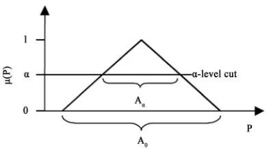
ceptually distinct, because fuzzy truth represents mem-bership in vaguely defined sets, not likelihood of some event or condition. Figure 4 shows a parameter P repre-sented as a triangular fuzzy number with support of A0.
The wider the support of the membership function, the higher the uncertainty. The fuzzy set that contains all elements with a membership of α ε [0,1] and above is called the α-cut of the membership function. At a resolu-tion level of α, it will have support of Aα. Higher the
[image:3.595.321.516.85.384.2]value of α, higher the confidence in the parameter.
Figure 3. Sketch for Monte Carlo Simulation method.
Figure 4. Fuzzy representation and Alpha cut.
The method is based on the extension principle, which implies that functional relationships can be extended to involve fuzzy arguments and can be used to map the de-pendent variable as a fuzzy set. The membership function is cut horizontally at a finite number of α-levels between 0 and 1. For each α-level of the parameter, the model is run to determine the minimum and maximum possible values of the output. This information is then directly used to construct the corresponding fuzziness (member-ship function) of the output which is used as a measure of uncertainty.
[image:3.595.325.520.409.517.2]Simulation uses an assumption that connected load will vary between 20% to 135% of rated data and are shown in Figure 5 and Figure 6. Above assumption can be rep-resented by a triangular distribution.
3. Simulation Results
In order to assess the results, two analyses were carried out: a spatial analysis, for which a measure of uncertainty was devised, and a point wise analysis, where the cumu-lative density probability function (CDF) for the MCS methods and the membership function for the FAC method of the output values were analysed.
3.1. Spatial Analysis
To evaluate the spatial distribution of uncertainty, meas-ure of uncertainty for the two methods is established. For the MCS method, such a measure is defined by the ratio of the standard deviation to the mean value, and for the FAC method the ratio of the 0.1-level support to the value for the membership function is equal to 1 (Refer Figure 7).
Fuzzy Membership function represen
0.00 0.20 0.40 0.60 0.80 1.00 1.20
0% 25% 50% 75% 100%
% of Load
M
em
b
er
sh
ip
f
u
n
cti
o
n
(M
F
)
tation
125% 150%
Figure 5. Fuzzy Membership function (MF) representation.
Figure 6. Probability density function representing limit a (20% in our case), upper limit b (130% on our case) and mode c (100%), where a < b and a ≤ c ≤ b.
Table 4 shows the calculated uncertainty values with FAC and MCS methods. It may be noted that uncertainty measure with FAC is much higher than that calculated using MCS method.
For understating this further, the output results are plotted for all the trails. Figure 8 is the histogram of sys-tem power losses for 500 trails using MCS method and Figure 9 is the scatter plot of MF vs. system power loss using FAC method. The output result range (variance) observed using FAC technique is much higher than that obtained from MCS method. It can be concluded that MCS method provides more reliable results compared to FAC method with less variance or uncertainty.
Figure 7. Measure of uncertainty for FAC technique.
Table 4. Calculated uncertainty values.
Method Basis (3.1) Uncertainty value
FAC Ratio of the 0.1-level support to the value at MF equal to 1 1.779
MCS Ratio of the Standard Deviation to the Mean Value 0.315
140 120 100 80 60 40 0.05
0.04
0.03
0.02
0.01
0.00
Power Loss
De
n
si
ty
Total Real Pow er Loss kW Total Reactiv e Pow er Loss kV A r V ariable
Histogram of Feeder Total Real Loss & Reactive Loss for 500 random trail
100.4 15.83 499 48.52 7.650 499 Mean StDev N
3.2. Pointwise Analysis
To evaluate the result obtained from spatial analysis fur-ther a point wise analysis is carried out and the algorithm is run for three cases shown in Table 5.
Figures 10-13 show the normalized Results obtained
300 250 200 150 100 50 0 1.0 0.8 0.6 0.4 0.2 0.0 X-Data MF 0.1 Reactiv e Loss kV
Real Loss kW V ariable Scatterplot o
[image:5.595.316.531.168.325.2]A r f MF vs Reactive Loss, Real Loss
[image:5.595.55.287.351.723.2]Figure 9. Scatter plot of MF vs. reactive, real power loss.
Table 5. Calculated uncertainty values.
Case Description FAC
Case
MCS Case
1
All connected load considered uncertain and varying independently as represented by Figure 5 and 6
F-1 R-1
2
Only one connected load connected to node 9 is assumed as uncertain and varying independently as represented by Figure 5 and 6
F-2 R-2
3
Three connected load connected to node 7, 9 & 12 are assumed as uncertain and varying
independently as represented by Figure 5 and 6
F-3 R-3 165 150 135 120 105 90 75 60 0.05 0.04 0.03 0.02 0.01 0.00 kW De n si ty
100.4 15.83 499 138.9 7.979 499 132.8 11.08 499
Mean StDev N
Real Loss case R-1 Real Loss case R-2 Real Loss case R-3
V ariable
Histogram of system Real Power Loss for Case R-1, R-2 & R-3
Figure 10. System real power loss for case R-1, R-2 & R-3.
shows that output range (variance) is more for Case 1, followed by Case 3 and minimum for Case 2 for each individual method. However when output is compared for two methods, the output from FAC method shows much more variance magnitude as compared to what obtained from MCS technique.
0.10 0.08 0.06 0.04 0.02 0.00
Reactive Loss case 1 Reactive Loss case 2 Reactive Loss case 3 Variable
Histogram of system Reactive Power Loss for Case R-1,R-2 & R-3
75.0 67.5 60.0 52.5 45.0 37.5 30.0 kVAr De n si ty
[image:5.595.56.287.354.722.2]48.52 7.650 499 67.14 3.857 499 64.17 5.354 499 Mean StDev N
Figure 11. System reactive power loss for case R-1, R-2 & R-3. 320 240 160 80 0 -80 0.035 0.030 0.025 0.020 0.015 0.010 0.005 0.000
133.4 89.02 22 140.1 11.94 22 136.5 25.85 22 Mean StDev N
Fuzzy Real Loss case F-1 Fuzzy Real Loss case F-2 Fuzzy Real Loss case F-3 Variable
Histogram of system Real Power Loss for Case F-1,F-2 & F-3
kW
De
n
si
ty
Figure12. System real power loss for case F-1, F-2 & F-3.
160 120 80 40 0 0.07 0.06 0.05 0.04 0.03 0.02 0.01 0.00
64.46 43.03 22 67.71 5.769 22 65.99 12.50 22
Mean StDev N F uzzy Reactiv e Loss case F -1 F uzzy Reactiv e Loss case F -2 F uzzy Reactiv e Loss case F -3 V ariable
Histogram of System Reactive Power Loss for Cases F-1,F-2 & F-3
kVAr
Den
si
ty
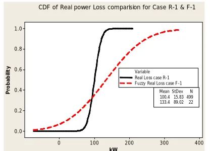
[image:5.595.313.529.357.525.2]Figure 14-16 show the cumulative density function (CDF) and normalized integrated fuzzy number plot for defined three cases. Results are comparable for Case 2 but the variance increases for Case 3 and is maximum for Case 1. The results also shows that variance difference between two techniques depends upon the number of uncertain input variables considered.
400 300 200 100 0 1.0 0.8 0.6 0.4 0.2 0.0 kW P ro b ab ilit y
100.4 15.83 499 133.4 89.02 22 Mean StDev N Real Los
Fuzzy R Variable CDF of Real power Loss comparision for
[image:6.595.67.278.368.518.2]s case R-1 eal Loss case F-1 Case R-1 & F-1
Figure 14. CDF of real power loss comparison for case R-1 & F-1. 200 180 0 16 140 120 100 80 60 1.0 0.8 0.6 0.4 0.2 0.0 kW P ro b a b ili ty
132.8 11.08 499 136.5 25.85 22 Mean StDev N
Real Loss case R-3 Fuzzy Real Loss case F-3 Variable
[image:6.595.66.277.553.709.2]CDF of Real power Loss comparision for Case R-3 & F-3
Figure 15 CDF of real power loss comparison for case R-3 & F-3. 17 160 150 140 130 120 110 0 1.0 0.8 0.6 0.4 0.2 0.0 kW P ro b a b ili ty
138.9 7.979 499 140.1 11.94 22 Mean StDev N Real Loss case R-2 Fuzzy Real Loss case F-2 Variable CDF of Real power Loss comparision for Case R-2 & F-2
Figure 16. CDF of real power loss comparison for case R-2 & F-2.
The reason of different variance can be explained with the fact that MCS considers random run for all connected load inputs, where as FAC technique takes two extreme values for all connected load values and envelops results for all extreme scenario together.
Simulation result for three cases shows that results ob-tained for single or limited input variables (i.e. case-3) are similar, however if an system has more uncertain input variables, MCS technique provides better results.
4. Conclusions
Fuzzy logic and probability are different ways of expressing uncertainty. While both fuzzy logic and probability the-ory can be used to represent subjective belief, fuzzy set theory uses the concept of fuzzy set membership (i.e., how much a variable is in a set), and probability theory uses the concept of subjective probability (i.e., how probable do I think that a variable is in a set). While this distinction is mostly philosophical, the fuzzy-logic-de-rived possibility measure is inherently different from the probability measure; hence they are not directly equiva-lent. Probability, which ranges from 0.0 to 1.0, is used to gauge the likelihood that some particular, well-defined state is or will be the case, under conditions of ignorance or chance. Fuzzy set membership function number, which also ranges from 0.0 to 1.0, indicates the degree to which an individual case or circumstance belongs to a fuzzy set. Here, values between 0.0 and 1.0 are a result of the in-herently imprecise nature of the definition of the fuzzy set, not ignorance or chance.
For the MCS approach large numbers of model runs are required (500 model run considered for this simula-tion), however FAC approach needed only 20 model runs. This is a drawback for MCS method due to its time con-suming characteristic. However, when simulation results are analyzed, result was found comparable, when uncer-tainty is on one input parameter. The variance increases, with increasing numbers of uncertain input variables. This is due to the fact that MCS considers random run for all connected load inputs, where as FAC technique takes two extreme values for connected load values.
It can be concluded that for more than one uncertain input variable, simulation result indicates that MCS method provides better output results compared to FAC, however takes more time due to number of runs. FAC provides an alternate method to MCS when addressing single or lim-ited input variables and is fast.
REFERENCES
[1] D. M. Falcao, “Load Estimation in Radial Distribution
Systems Using Neural Networks and Fuzzy Set
Tech-niques,” Power Engineering Society Summer Meeting,
doi:10.1109/PESS.2001.970195
[2] C.-W. Liu, C.-S. Chang and M.-C. Su, “Neuro-Fuzzy
Net-works for Voltage Security Monitoring Based on
Syn-cronized Phasor Measurements,” IEEE Transactions on
Power Systems, Vol. 13, No. 2, 1998, pp. 326-332.
doi:10.1109/59.667346
[3] I. J. Ramirez-Rosad and J. A. Dominguez-Navarro,
“Possi-bilistic Model Based on Fuzzy Sets for the Multiobjective Optimal Planning of Electric Power Distribution Networks,”
IEEE Transactionson Power Systems, Vol. 19, No. 4, 2004,
pp. 1801-1810. doi:10.1109/TPWRS.2004.835678
[4] V. Kumar and M. Schuhmacher, “Fuzzy Uncertainty Ana-
lysis in System Modeling,” European Symposium on Com-
puter Aided Chemical Engineering, Vol. 20, 2005, pp. 391-
396. doi:10.1016/S1570-7946(05)80187-7
[5] A. J. Abebe, V. Guinot and D. P. Solomatine, “Fuzzy
Al-pha-Cut vs. Monte Carlo Techniques in Assessing
Uncer-tainity in Model Parameters,” Proceedings of the 4th
In-ternational Conference on Hydro Informatics, Iowa City, 23-27 July 2000, pp. 1-8.
[6] M. S. Thomas, R. Ranjan and R. Raina, “Fuzzy Modeled
Load Flow Solution for Unbalanced Radialpower
Distri-bution System,” Proceedings of the IASTED International
Conference, Crete, 22-24 June 2011, pp. 153-159.
doi:0.2316/P.2011.714-003
[7] D. Thukram, H. M. W. Banda and J. Jerome, “A Robust
Three Phase Power Flow Algorithm for Radial
Distribu-tion Systems,” Journal of Electrical Power Systems
Re-search, Vol. 50, No. 3, 1999, pp. 227-236.