ISSN Online: 2152-7261 ISSN Print: 2152-7245
Machine Learning Approaches to Predict
Default of Credit Card Clients
Ruilin Liu
University of Southern California, Los Angeles, CA, USA
Abstract
This paper compares traditional machine learning models, i.e. Support Vec-tor Machine, k-Nearest Neighbors, Decision Tree and Random Forest, with Feedforward Neural Network and Long Short-Term Memory. We observe that the two neural networks achieve higher accuracies than traditional mod-els. This paper also tries to figure out whether dropout can improve accuracy of neural networks. We observe that for Feedforward Neural Network, ap-plying dropout can lead to better performances in certain cases but worse performances in others. The influence of dropout on LSTM models is small. Therefore, using dropout does not guarantee higher accuracy.
Keywords
Machine Learning, Feedforward Neural Network, Long Short-Term Memory, Dropout
1. Introduction
Neural network can explore the relationship among input features and corres-ponding labels, so it is suitable for complex machine learning problems. On the other hand, other machine learning models such as linear regression or Support Vector Machine (SVM) [1] can solve simpler problems more efficiently. There-fore, after analyzing specific problems, one should answer the question of “is neural network really necessary in this case?”
Moreover, there are different models within the category of “neural network”. Feedforward Neural Network uses neurons in the same layer together at the same time to calculate neurons in the next layer. Besides their difference in weights, neurons are “parallel” in this process. On the contrary, Recurrent Neur-al Network is a useful model for sequentiNeur-al dataset. It Neur-allows previous inputs to influence the processing of future inputs. The difference in accuracy between How to cite this paper: Liu, R.L. (2018)
Machine Learning Approaches to Predict Default of Credit Card Clients. Modern Economy, 9, 1828-1838.
https://doi.org/10.4236/me.2018.911115
Received: September 7, 2018 Accepted: November 16, 2018 Published: November 19, 2018
Copyright © 2018 by author and Scientific Research Publishing Inc. This work is licensed under the Creative Commons Attribution International License (CC BY 4.0).
http://creativecommons.org/licenses/by/4.0/ Open Access
these two networks should be compared [2]-[8].
We discuss previous research in Section 2, model description in Section 3, da-taset description and experiment results in Section 4, conclusion in Section 5 and potential future work in Section 6.
2. Related Works
Yeh [2] randomly divided 25,000 payment data into a training set and a testing set. Then they chose six data mining methods—Logistic Regression, Discrimi-nant Analysis (Fisher’s rule), Naïve Bayes, kNN, Decision Tree and (Feedfor-ward) Neural Network. The error rate of each model on testing set was recorded. Accuracies were known by using 1 − (error rate). kNN returned the highest ac-curacy of 0.84. Feedforward Neural Network and Decision Tree both returned second highest accuracy of 0.83. Discriminant Analysis returned the lowest ac-curacy of 0.74. From this paper, one could observe that neural network is not guaranteed to have better performance than other simpler models, and one of the traditional models, kNN, was able to achieve higher accuracy than neural network. However, they did not apply the technique of dropout on their neural network model. Also, Long Short-Term Memory [3], a model that is widely ap-plied now, was not considered. In neural networks, there is an “epochs” para-meter that determines how many times a sample is fed into the model, but this parameter was not included in Yeh [2]. To have clearer comparisons between neural networks and traditional models, a research that includes these factors is needed.
3. Model Description
3.1. k-Nearest Neighbors
k-Nearest Neighbors (kNN) [4] stores all training samples (including their fea-tures and labels) in a space according to its metrics without processing or calcu-lation. When the model receives an object to be predicted, it puts the new object into that space (also according to the metrics). The model then makes prediction by looking at k nearest neighbors to the new object. Usually, the prediction is the label that occurs the most among those k samples.
This model determines a sample’s label based on nearby samples with known labels, so it does not “get trained” but only memorizes. To truly train a boundary that separates two categories and can be used for future predictions, Support Vector Machine is a classical model to choose [5].
3.2. Support Vector Machine
Support Vector Machine (SVM) first puts all samples in a space. It represents two categories as 1 and −1. Then it finds two parallel hyperplanes, and each hyperplane limits the boundary of one category. With normalized dataset, these two hyperplanes are expressed as w x b, + = +1 and w x b, + = −1, where w is the normal vector of the hyperplanes, x is the input vector, and b is the
stant. The training process is to find w so that the distance between these two hyperplanes is maximized. When it receives a new input vector xi, it labels it 1 if
, 1
w xi b+ ≥ , or −1 if w xi b, + ≤ −1.
If the dataset cannot be perfectly separated, the model increases the dimension of the dataset. SVM tries to find the dimension that is high enough and the da-taset can be perfectly separated. Then, linear SVM can be applied.
SVM draws boundary in the sample space, and a different approach of catego-rizing is to make a series of comparisons between trained numbers and the val-ues of explanatory variables. This is what Decision Tree does [6].
3.3. Decision Tree and Random Forest
Decision Tree is a tree graph with “if” statements. Each if-statement divides the samples into two branches. Samples that satisfy the if-statements go to one di-rection, and samples that do not satisfy go to the other direction. The training process is to find out if-statements that can make largest divisions.
Still, this model needs to be restricted. If the depth of tree is large, those if-statements would gradually become very narrow because they need to separate more similar samples into different direction. This means too much training and overfitting [6]. Therefore, the depth of the tree is often limited. This can be achieved by setting either the maximum depth directly, or the minimum number of samples required in leaf nodes (suppose node A contains only 20 samples and the minimum number of samples required is 30, then node A should not exist, and its parent should be the leaf node).
To further avoid overfitting, Random Forest repeatedly selects some random samples with replacement, and train multiple Decision Trees. When it receives a new sample, all those trees make predictions and do majority voting to deter-mine the label of the new sample.
3.4. Neural Network & Dropout
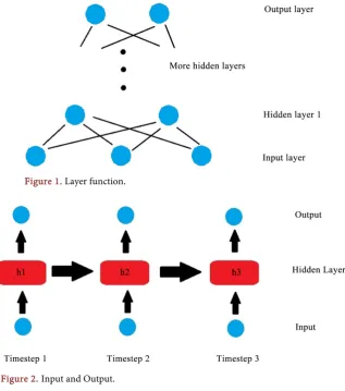
Neural Network consists of an input layer, some hidden layers and an output layer. As shown in Figure 1, the input layer takes features in the dataset as input. Then, these neurons together are used to compute each of the neuron in the next layer according to the weights of their connections (each bridge between two neurons has its unique weight). Each layer also has an activation function. This function determines the value a neuron passes to the next layer according to the value it receives from the previous layer. The final layer is the output layer.
However, one problem of the Neural Network is that when the number of layers and neurons is large, there could be many connections between neurons. If a model considers all connections and trains all the weights every time, that model may become too complicated while training. This results in overfitting in the model. Dropout is a useful way to avoiding overfitting. When the previous layer passes values to the next layer, it randomly ignores certain number of neu-rons and all their connections to the next layer (according to the dropping rate
parameter). This decreases the number of neurons for each layer and prevents too much training and reduces overfitting.
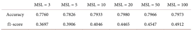
The Neural Network described above ignores the sequential relationships of inputs. In real world problems, previous events can potentially affect future events, so it is valuable to take time sequence into account while doing machine learning. Recurrent Neural Network is a suitable model for this.
3.5. Recurrent Neural Network & Long Short-Term Memory
Recurrent Neural Network (RNN) can reflect the sequential relationship among inputs. The hidden layer used to process previous inputs is passed to next den layers, which are used to process future inputs. Therefore, by training hid-den layers, previous inputs can affect how the model processes future inputs (Figure 2).Long Short-Term Memory (LSTM) is an advanced architecture of RNN. RNN may have gradient vanishing or explosion when timestep is long. LSTM has a cell state that processes the inputs, and the cell state is also passed to the next timestep. The forget gate uses a sigmoid function to determine what proportion of cell state is kept. With the forget gate, the gradient is guaranteed to be in an ideal range.
[image:4.595.214.532.369.729.2]Figure 1. Layer function.
Figure 2. Input and Output.
4. Dataset & Experiments
This dataset is provided by I-Cheng Yeh [2], from Department of Information Management, Chung Hua University, Taiwan. It is accessed from UCI Machine Learning Repository. It contains 30,000 samples of credit information and whether default occurs. The explanatory variables include “the amount of credit, gender (1 = male; 2 = female), education (1 = graduate school; 2 = university; 3 = high school; 4 = others), marital status (1 = married; 2 = single; 3 = others), age, history of delayed payment from April to September, 2005, amount of bill state-ment from April to September, 2005, and amount paid from April to September, 2005”. 6636 of 30,000 samples have default payments, 23,364 do not. The 30,000 samples are randomly shuffled, and after shuffling, the top 10,000 samples are chosen. The top 8500 samples are used as training set, and the rest 1500 samples are used as testing set. The data has been normalized to mean of 0 and variance of 1.
4.1. F1-Score
Accuracy is Number of correct predictions
Number of samples . When the dataset is imbalanced,
accuracy may not be sufficient because simply predicting all samples to be the major class can still get high accuracy.
In such situation, a good metrics to use is f1-score. F1-score is calculated by 2 precision recall
precision recall
∗ ∗
+ , where precision is
True Positives
True Positives False Positives+ , and
recall is True Positives
True Positives False Negatives+ . Precision measures a model’s ability to
correctly identify positive samples, and recall measures the proportion of tive samples that are identified. F1-score ranges from 0, cannot make true posi-tive prediction, to 1, being correct in all predictions.
In this dataset, 77.88% of samples are negative. While this paper still focuses on accuracies, f1-scores are also be measured as references to guarantee that models are not blindly guessing samples to be negative. If a model has strong tendency to make negative predictions, its recall will be low, so it will return a low f1-score (Tables 1-3).
When the kernel is “RBF” and C = 1, the accuracy, 0.804, is the highest among all results. The corresponding f1-score is 0.4520. The f1-scores of “RBF” kernel is generally higher than the scores of “Poly” kernel.
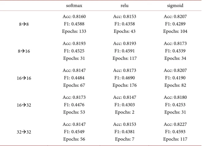
Random Forest is better than Decision Tree since it reduces overfitting, and both accuracies and f1-scores reflect this. In this experiment, when MSL is 10 or 20, the accuracy is 0.8000, slightly higher than the accuracy of the previous Deci-sion Tree which has MSL set to 20. When MSL > 5, there is no significant dif-ference on accuracies. The f1-score when MSL = 10 is 0.4544, and the f1-score when MSL = 20 is 0.4425, so there is little difference between setting MSL to 10 or 20.
Table 1. SVM.
C = 0.01 C = 0.1 C = 1 C = 10 C = 50 C = 100 Poly acc: 0.7700 0.7813 0.7913 0.7900 0.7893 0.7846
[image:6.595.208.542.209.257.2]Poly f1: 0.0247 0.1676 0.3372 0.3939 0.3984 0.3984 RBF acc: 0.7626 0.7940 0.8040 0.8013 0.7973 0.7806 RBF f1: 0.0000 0.4054 0.4520 0.4638 0.4658 0.4525
Table 2. KNN.
k = 3 k = 5 k = 10 k = 20 k = 50 k = 100 Accuracy 0.7760 0.7826 0.7933 0.7980 0.7966 0.7973 f1-score 0.4384 0.4349 0.4077 0.4077 0.3920 0.3704
Table 3. Decision Tree: (min_samples_leaf is denoted by “MSL”).
MSL = 3 MSL = 5 MSL = 10 MSL = 20 MSL = 50 MSL = 100 Accuracy 0.7760 0.7826 0.7933 0.7980 0.7966 0.7973
f1-score 0.3697 0.3906 0.4046 0.4465 0.4547 0.4912
4.2. Feedforward Neural Network
In this paper, “relu”, “softmax” and “sigmoid” activation functions will be com-pared. There are two layers with the same activation function. The output layer has 2 neurons and “softmax” as activation function, so that the output is a probability distribution.
4.3. Feedforward Neural Network without Dropout
In Table 4, numbers on the leftmost column represent the number of neurons in corresponding layers (i.e., “8→8” means a Dense layer with 8 neurons, followed by another Dense layer with 8 neurons). The “Epochs” parameter varies from 1 to 400 for each model, and the value represents the “Epochs” which returns the highest accuracy for that model. These highest accuracies and their correspond-ing f1-scores and “Epochs” are compared in the followcorrespond-ing table.
According to the accuracies and f1-scores, “sigmoid” activation function out-performs “softmax” and “relu”. For 4 out of 5 cases, “sigmoid” has the highest accuracies. The highest accuracy, 0.8227, also occurs in “sigmoid” when there are 32 neurons in both layers and training samples are fed into the model 117 times.
However, the f1-scores of “sigmoid” models are lower than those of “softmax” and “relu”, so for heavily imbalanced dataset, the other two activation functions are better choices.
4.4. Feedforward Neural Network with Dropout: (Using Sigmoid)
In this experiment, a dropout function is set between the second last layer and [image:6.595.207.542.291.343.2]the output layer. Accuracies and f1-scores with dropout are compared with those without dropout (Tables 5-7).
Accuracy & f1-score table for Dense(8)→Dense(8)→Dense(2), first two layers using “sigmoid” activation
Accuracy & f1-score table for Dense(16)→Dense(16)→Dense(2), first two layers using “sigmoid” activation
Accuracy & f1-score table for Dense(32)→Dense(32)→Dense(2), first two layers using “sigmoid” activation
When each layer has only 8 neurons, using dropout causes decrease in accura-cies and increase in f1-scores at the beginning, but as the dropout rate becomes 0.3, f1-score decreases too. Dense(16)→Dense(16) →Dense(2) shows better performance after applying dropout. Having higher dropout rate increases both accuracies and f1-scores. When each layer has 32 neurons and dropout is added, the model can still get high accuracies (higher than 0.82) and high f1-scores (higher than 0.45), both are relatively better than other two models.
Therefore, dropout in Feedforward Neural Network can be useful only when there are larger numbers of neurons in each layer. The reason might be that, if the number of neurons is already small, like 8 neurons per layer, dropping neu-rons and connections could make the model lack of necessary information.
4.5. LSTM without Dropout
In the following models, all layers use “sigmoid” as activation function since it returns high accuracies in Feedforward Neural Network. A feedforward Dense layer with 2 neurons is also added after the output layer of LSTM. The “Adam” optimization algorithm is used during training. “Epochs” also ranges from 1 to 400, depending on when each model returns its highest accuracy (Table 8).
According to the results, LSTM models have lower accuracies than Feedfor-ward Neural Network. Using “sigmoid” activation function, 3 FeedforFeedfor-ward Neural Network models have accuracies higher than 0.82, but among these five LSTM models, none of them have accuracies higher than that. Also, there are no observable improvements of f1-scores while using LSTM models.
4.6. LSTM with Dropout
Three models, LSTM(8)→LSTM(8)→Dense(2), LSTM(16)→LSTM(16)→ Dense(2) and LSTM(32)→LSTM(32)→Dense(2) are chosen. Their accuracies and f1-scores with and without dropout are compared. A dropout technique is set between the second last layer and the output layer. Other settings are the same as previous LSTM models (Tables 9-11).
Accuracy & f1-score table for LSTM(8)→LSTM(8)→Dense(2), first two layers using “sigmoid” activation
Accuracy & f1-score table for LSTM(16)→LSTM(16)→Dense(2), first two layers using “sigmoid” activation
Accuracy & f1-score table for LSTM(32)→LSTM(32)→Dense(2), first two layers using “sigmoid” activation
Table 4. Corresponding f1-scoresand “Epochs”.
softmax relu sigmoid
88
Acc: 0.8160 F1: 0.4588 Epochs: 133 Acc: 0.8153 F1: 0.4358 Epochs: 43 Acc: 0.8207 F1: 0.4289 Epochs: 104
816
Acc: 0.8193 F1: 0.4525 Epochs: 31 Acc: 0.8193 F1: 0.4591 Epochs: 117 Acc: 0.8173 F1: 0.4339 Epochs: 34
1616
Acc: 0.8147 F1: 0.4484 Epochs: 67 Acc: 0.8173 F1: 0.4690 Epochs: 176 Acc: 0.8207 F1: 0.4190 Epochs: 82
1632
Acc: 0.8173 F1: 0.4476 Epochs: 53 Acc: 0.8147 F1: 0.4303 Epochs: 2 Acc: 0.8180 F1: 0.4253 Epochs: 31
3232
[image:8.595.211.539.361.458.2]Acc: 0.8147 F1: 0.4549 Epochs: 56 Acc: 0.8153 F1: 0.4381 Epochs: 7 Acc: 0.8227 F1: 0.4593 Epochs: 117
Table 5. Accuracy & f1-score.
Accuracy F1-score Epochs
Without dropout 0.8207 0.4289 104
Dropout rate = 0.1 0.8193 0.4366 34
Dropout rate = 0.2 0.8193 0.4435 188
Dropout rate = 0.3 0.8160 0.4153 44
Table 6. Accuracy & f1-score.
Accuracy F1-score Epochs
Without dropout 0.8207 0.4190 82
Dropout rate = 0.1 0.8173 0.4315 58
Dropout rate = 0.2 0.8213 0.4440 96
Dropout rate = 0.3 0.8227 0.4637 139
Table 7. Accuracy & f1-score.
Accuracy F1-score Epochs
Without dropout 0.8227 0.4593 117
Dropout rate = 0.1 0.8246 0.4509 133
Dropout rate = 0.2 0.8220 0.4649 324
Dropout rate = 0.3 0.8200 0.4328 76
[image:8.595.211.540.493.590.2] [image:8.595.209.542.626.729.2]Table 8. LSTM models.
[image:9.595.208.541.235.324.2]Accuracy F1-score Epochs LSTM(8)LSTM(8)Dense(2) 0.8180 0.4371 85 LSTM(8)LSTM(16)Dense(2) 0.8173 0.4244 82 LSTM(16)LSTM(16)Dense(2) 0.8180 0.4324 59 LSTM(16)LSTM(32)Dense(2) 0.8153 0.4241 70 LSTM(32)LSTM(32)Dense(2) 0.8193 0.4503 106
Table 9. Accuracy & f1-score.
Accuracy F1-score Epochs
Without dropout 0.8180 0.4371 85
Dropout rate = 0.1 0.8213 0.4417 129
Dropout rate = 0.2 0.8180 0.4485 269
Dropout rate = 0.3 0.8233 0.4421 152
Table 10. Accuracy & f1-score.
Accuracy F1-score Epochs
Without dropout 0.8180 0.4324 59
Dropout rate = 0.1 0.8193 0.4655 119
Dropout rate = 0.2 0.8187 0.4494 123
Dropout rate = 0.3 0.8193 0.4547 168
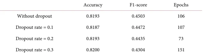
Table 11. Accuracy & f1-score.
Accuracy F1-score Epochs
Without dropout 0.8193 0.4503 106
Dropout rate = 0.1 0.8187 0.4472 107
Dropout rate = 0.2 0.8193 0.4435 73
Dropout rate = 0.3 0.8200 0.4304 151
Using dropout does not lead to significantly better performances. In most cases, accuracies for LSTM models are around 0.82. An advantage over Feed-forward Neural Network is that f1-scores of LSTM are stable. After applying dropout, for Feedforward Neural Network there are some sudden decreases in f1-scores. Such phenomena are not observed on LSTM models. Since both accu-racies and f1-scores are stable, it is fair to conclude that dropout does not have strong influence on LSTM. An explanation is that a LSTM model already has complicated connections within and between timesteps, so dropping several connections cannot be reflected.
[image:9.595.208.539.360.449.2] [image:9.595.210.540.484.574.2]5. Conclusions
Traditional machine learning models are only able to achieve accuracy of 0.8040, which is achieved by SVM. The highest accuracy of neural network is 0.8246, by using Dense(32)→Dense(32)→Dense(2), dropout rate = 0.1, “sigmoid” as acti-vation function. For LSTM, LSTM(8)→LSTM(8)→Dense(2), dropout rate = 0.3, “sigmoid” as activation function achieves accuracy of 0.8233, which is also better than the best traditional model. Looking at f1-scores, many of neural networks’ f1-scores are around 0.44, while Random Forest and SVM using “rbf” kernel can reach 0.45. However, the difference on accuracies is more significant.
Therefore, unlike the research of Yeh [2] shown in Section 2, neural networks outperform traditional models, except for situations when the research strongly focuses on positive predictions (False Negative is dangerous and high f1-score is required).
For Feedforward Neural Network, using dropout is sometimes efficient for better performance. The accuracies and f1-scores for Dense(16)→Dense(16) and Dense(32)→Dense(32) are generally improved. Therefore, when using feedfor-ward neural network, dropout can be helpful when the number of neurons per layer is not small.
For LSTM, using dropout does not make significant difference. The accuracies and f1-scores are all close to the results without using dropout. Still, dropout can be applied if one tries to avoid False Negative and focuses on f1-score. Unlike the results of Feedforward Neural Network models, using dropout on LSTM pre-vents sudden decrease in f1-scores.
A noticeable point is that LSTM models perform worse than Feedforward Neural Network. Generally, people would prefer LSTM and consider it as ad-vanced architecture of neural network, but experiments in this paper show that LSTM get similar f1-scores and even lower accuracies compared to Feedforward Neural Network. Future work is needed to explain this abnormal phenomenon and give a clear boundary of whether to use LSTM or not.
Conflicts of Interest
The author declares no conflicts of interest regarding the publication of this pa-per.
References
[1] Weston, J. (n.d.) Support Vector Machine (and Statistical Learning Theory) Tutori-al. NEC Labs America.
http://www.cs.columbia.edu/~kathy/cs4701/documents/jason_svm_tutorial.pdf
[2] Yeh, I.C. and Lien, C.H. (2009) The Comparisons of Data Mining Techniques for the Predictive Accuracy of Probability of Default of Credit Card Clients. Expert Systems with Applications, 36, 2473-2480.
https://doi.org/10.1016/j.eswa.2007.12.020
[3] Hochreiter, S. and Schmidhuber, J. (1997) Long Short-Term Memory. Neural Computation, 9, 1735-1780. https://doi.org/10.1162/neco.1997.9.8.1735
[4] Cover, T.M. and Hart, P.E. (1967) Nearest Neighbor Pattern Classification. IEEE Transactions on Information Theory, IT-IS, 21-27.
[5] Cortes, C. (1995) Support-Vector Networks. Machine Learning, 20, 273-297.
https://doi.org/10.1007/BF00994018
[6] Quilan, J.R. (1986) Induction of Decision Trees. Machine Learning, 1, 81-106.
https://doi.org/10.1007/BF00116251
[7] Rosenblatt, F. (1958) The Perceptron: A Probabilistic Model for Information Sto-rage and Organization in the Brain. Psychological Review, 65, 386-408.
[8] Breiman, L. (2001) Random Forests. Machine Learning, 45, 5-32.
https://doi.org/10.1023/A:1010933404324