Using Two Levels DWT with Limited Sequential Search
Algorithm for Image Compression
Mohammed Mustafa Siddeq
Software Engineering Department, Technical College, Kirkuk, Iraq. Email: [email protected]
Received November 10th,2011; revised December 12th, 2011; accepted December 21st, 2011
ABSTRACT
In this paper introduce new idea for image compression based on the two levels DWT. The low-frequency sub-band is minimized by using DCT with the Minimize-Matrix-Size-Algorithm, which is converting the AC-coefficients into array contains stream of real values, and then store the DC-coefficients are stored in a column called DC-Column. DC-Column is transformed by one-dimensional DCT to be converted into T-Matrix, then T-Matrix compressed by RLE and arithmetic coding. While the high frequency sub-bands are compressed by the technique; Eliminate Zeros and Store Data (EZSD). This technique eliminates each 8 × 8 sub-matrix contains zeros from the high frequencies sub-bands, in another hands store nonzero data in an array. The results of our compression algorithm compared with JPEG2000 by using four different gray level images.
Keywords: DWT; DCT; Minimize-Matrix-Size-Algorithm; LSS-Algorithm; Eliminate Zeros and Store Data
1. Introduction
Digital representation of image has created the need for efficient compression algorithms that will reduce the sto- rage space and the associated channel bandwidth for the transmission of images. Wavelet transforms have become more and more popular in the last decade in the field of image compression [1]. They have an advantage over the block-based transforms such as Discrete Cosine Trans- form (DCT) which exhibits blocking artifact. Wavelets with compact support provide a versatile alternative to DCT [2]. The groundbreaking single-wavelet examples provided multiresolution function-approximation bases formed by translations and dilations of a single approxi- mation functions and detail functions. In the last years multi-wavelets, which consist of more than one wavelet have attracted many researchers [3]. Certain properties of wavelets such as orthogonally, compact support, linear phase, and high approximation/vanishing moments of the basis function, are found to be useful in image compres- sion applications. Unfortunately, the wavelets can never possess all the above mentioned properties simultane- ously [4]. To overcome these drawbacks, more than one scaling function and mother wavelet function need to be used. Multi-wavelets posses more than one scaling func- tion offer the possibility of superior performance and high degree of freedom for image processing applications, compared with scalar wavelets. Multi-wavelets can achi- eve better level of performance than scalar wavelets with
similar computational complexity [5]. In the case of non- linear approximation with multi-wavelet basis, the multi- wavelet coefficients are effectively “reordered” accord- ing to how significant they are in reducing the approxi- mation error [6]. The JPEG2000 is a new image com- pression standard, recently, introduced by Joint Picture Experts Group [7]. In addition to its improved compres- sion ability, JPEG2000 provides many features which are of high importance to many applications in which the quality and performance criteria are crucial, such appli- cations are scanning, remote sensing, recognition, medi- cal imaging [8]. Comparative test results have shown that the JPEG2000 is superior to existing still image com- pression standards [9]. A review paper as well as com- parative works with the existing compression standards can be found in the literature. JPEG2000 start with dis- crete wavelet transform to the source image data. The coefficients obtained from the wavelet transform are then quantized and entropy coded, before forming the output bit stream. JPEG2000 standard supports both lossy and lossless compression. This depends on the wavelet trans- form and the quantization applied [10].
This research introduces a new idea for image compre- ssion depending on two transformations with Minimize- Matrix-Size algorithm and using LSS-Algorithm for de-coding.
2. Proposed Compression Algorithm
tions. First transformation is two levels DWT, converts the images into seven sub-bands, and the second trans- formation is two dimensional DCT applied on each “2 × 2” block of data from low-frequency sub-band “LL2”. The DCT is very important for our approach sharing with DWT for obtains more high-frequencies domains. DCT plays main role for converting sub-band “LL2” into DC- coefficients and AC-coefficients, DC-coefficients stored in a column called DC-Column, while AC-coefficients are stored in the AC-Matrix, and then applied Minimize- Matrix-Size Algorithm on the AC-Matrix to convert AC- coefficients into array, as shown in Figure 1.
2.1. Using Discrete Wavelet Transform (DWT)
Wavelet transform has the capability to offer some in-
formation on frequency-time domain simultaneously. In this transform, time domain is passed through low-pass and high-pass filters to extract low and high frequencies respectively. This process is repeated for several times and each time a section of the signal is drawn out. DWT analysis divides signal into two classes (i.e. Approxima-
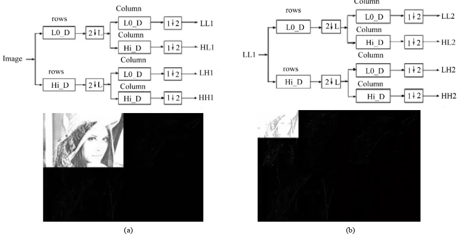
tion and Detail) by signal decomposition for various fre- quency bands and scales [11]. DWT utilizes two function sets: scaling and wavelet which associate with low and high pass filters orderly. Such a decomposition manner bisects time separability. In other words, only half of the samples in a signal are sufficient to represent the whole signal, doubling the frequency separability. Figure 2 shows two level decomposition the “Lena” image.
The wavelet decomposition has some important fea-
Each 2
2 square converted into DC-Column and AC-Matrix Sub-band “LL2”Transformed by DCT for each (2 x 2)
Block
123 125 126 100 109 110 … …
Minimize Matrix size Algorithm
0 0 1 -1 0 1 0 0 0 -1 -1 1 1 -2 -1 0 1 0 … …
Arithmetic Coding
Produce T-Matrix LL2
HL
2HL
1(Ignored) LH2 HH2
LH
1HH
1 (Ignored) (Ignored)RLE and Arithmetic Coding EZSD and
[image:2.595.107.490.284.447.2]Arithmetic Coding
Figure 1. Applied Minimize-Matrix-Size algorithm on the LL2 sub-band.
(a) (b)
[image:2.595.63.528.480.718.2]tures; many of the coefficients for the high-frequency components (LH, HL and HH) are zero or insignificant [12]. This reflects the fact that the much of the important information is in “LL” sub-band. The DWT is a good choice of transform accomplishes a de-correlation for the pixels, while simultaneously providing a representation in which most of the energy is usually restricted to a few coefficients [13], while other sub-bands (i.e. LH1, HL1 and HH1) are ignored. This is the key for achieving a high compression ratio. The Daubechies Wavelet Trans- form family has ability to reconstructs images, by using just LL1 without need for other high-frequencies. But this leads for obtains less image quality.
2.2. Using Discrete Cosine Transform (DCT)
DCT is the second transformation is used in this research, which is applies on each “2 × 2” block from “LL2” sub-band as show in Figure 3.
DCT produce DC value and AC coefficients. Each DC value is stored in the DC-Column, and the other three AC coefficients are stored in the AC-Matrix.
2.2.1. Quantization Level1
In the above Figure 3, “Quantization level1” is used to reduce size of the data for LL2, by select the ratio of maximum value for LL2 as shown in the following equa-tions:
21 Quality max LL
Q
(1)2 2 LL LL round 1 Q
(2)
“Quality” value is used in Equation (1), affects in the image quality. For example “Quality = 0.005”, this means compute 0.5% from maximum value in LL2 to be divided by all values in LL2. This process helps the LL2 values to be more converging (i.e. more correlated). In
another hands this quantization process leads to obtains low image quality, if the Quality > 1%.
2.2.2. Quantization Level2
Each “2 × 2” coefficients from LL2 is transformed by DCT and then divided by “Q2”, using matrix-dot-division. This process removes insignificant coefficients and in-creasing the zeros in the transformed LL2. The “Q2” can be computed as follows [4]:
1, if 1 and 1
2 ,
, if 1 and 1
i j
Q i j
i j R i j
(3)
2.2.3. Using Two Dimensional DCT
The energy in the transformed coefficients is concen- trated about the top-left corner of the matrix of coeffi- cients. The top-left coefficients correspond to low fre-
Figure 3. LL2 sub-band quantized and transformed by DCT
for each 2 × 2 blocks.
quencies: there is a “peak” in energy in this area and the coefficients values rapidly decrease to the bottom right of the matrix, which means the higher-frequency coeffi- cients [3].
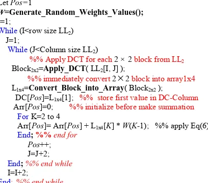
The DCT coefficients are de-correlated, which means that many of the coefficients with small values can be discarded without significantly affecting image quality. A compact matrix of de-correlated coefficients can be compress much more efficiently than a matrix of highly correlated image pixels [4]. The following equations il- lustrated DCT and Inverse DCT function for two-dimen- sional matrices “2 × 2”:
3 3
0 0 ,
2 1 π 2 1 π
, cos cos
4 4
x y
C u v a u a v
x u y
f x y
v
(4)where
1, 02
a u for u , a u
1, for u0
3 3
u 0 v 0
,
(2 1) π (2 1) π
, cos cos
4 4
f x y
x u y
a u a v C u v
v
[image:3.595.321.522.87.328.2] [image:3.595.310.541.521.676.2]DCT. The DCT becomes increasingly complicated to calculate for the larger block sizes, for this reason in this paper used “2 × 2” block to be transformed by DCT, whereas a DWT will be more efficiently applied to the complete images and produce good compression ratio.
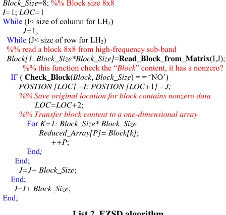
2.3. Apply Minimize-Matrix-Size Algorithm
The DWT and DCT it’s used for increasing number of the high-frequency coefficients, but this is not enough in our approach, for this reason in this research introduces a new algorithm for minimizing the size of AC-Matrix into array. This algorithm based on the Random-Weights- Values. The following equation represents converting AC-Matrix into array:
( ) (1) * ( ,1) (2) * ( , 2) (3) * ( ,3)
Arr L W AC L W AC L
W AC L
(6)
Note: “AC” is represents AC-Matrix.
L = 1, 2, 3,··· Column size of AC-Matrix.
The “W” in Equation (6) is represents Random-
Weights-Values, generated by random function in MAT- LAB language, the “W” values between {0···1}, for example: W = {0.1, 0.65, 0.423}. The Random-Weights-
Values are multiply with each row from AC-Matrix, to produce single floating point value “Arr”, this idea it’s similar to the neural network equations. The neural net- works equations; multiplies the updated weights values with input neurons to produce single output neuron [14]. Minimize-Matrix-Size Algorithm is shown in the fol- lowing List 1:
Before apply the Minimize-Matrix-Size algorithm, our compression algorithm computes the probability of the AC-Matrix. These probabilities are called Limited-Data, which is used later in decompression algorithm, the Lim- ited-Data stored in the header for compressed file. Be- cause these data uncompressible.
Let Pos=1
W=Generate_Random_Weights_Values();
I=1;
While (I<row size LL2) J=1;
While (J<Column size LL2)
%% Apply DCT for each 2 ×2 block from LL2
Block2x2=Apply_DCT( LL2[I, J] ); %% immediately convert 2
2 block into array1x4L1x4=Convert_Block_into_Array( Block2x2 );
DC[Pos]=L1x4[1]; %% store first value in DC-Column Arr[Pos]=0; %% initialize before make summation
ForK=2 to 4
Arr[Pos]= Arr[Pos] + L1x4[K] * W(K-1); %% apply Eq(6) End; %% end for
Pos++;
J=J+2; End; %% end while
I=I+2;
End; %% end while
List 1. Minimize-Matrix-Size algorithm.
Figure 4 illustrates probability of data for a matrix. The final step in this section is; Arithmetic coding, which takes stream of data and convert it into single floating point value. These output values in the range less than one and greater than zero, when decoded this value getting exact stream of data. The arithmetic coding need to compute the probability of all data and assign range for each data, the range value consist from Low and High value [3,4].
2.4. T-Matrix Coding
The DC-Column contains integer values, these values are obtained from pervious section (See Section 2.2). The arithmetic coding unable to compress this column, be- cause these values are correlated, for this reason DC- Column partitioned into 128-parts, and each partition is transformed by DCT (See Equation (1)) as a one-dimen- sional array by using u = 0 and x = 0 in Equation (1) to
be one-dimensional DCT and then using quantization process for each row, as shown in the following equa- tion:
1
2Q n Q n (7)
Note: n= 2,3,···, 128.
The initial value of Q(1) = 12.8.
The first value in above Equation (7) is Q(1) = 12.8,
because the length of each row is 128. Each 128 values are transformed and stored as a row in the matrix called Transformed-Matrix (T-Matrix). This part of our com- pression algorithm it’s look like JPEG technique, as shown in Figure 5. The idea for using T-Matrix, this is because we need to increase number of zeros or insig- nificant and makes values more de-correlated, this process increases compression ratio. Each row from T-Matrix consists of; DC value and stream of AC coefficients, now we need to scan T-Matrix column-by-column for con- verting it into one-dimensional array, and then compress it by Run Length Encoding (RLE) and arithmetic coding.
RLE it counts the repeated coefficients, and then refers to the repeated coefficients by a value, this process re- duce the length of the repeated data, then applying the arithmetic coding to convert these reduced data into bits. For more information about RLE and Arithmetic coding is in [3,4].
2.5. Applied Eliminate Zeros and Store Data (EZSD)
[image:4.595.59.263.536.715.2]Figure 4. Illustrates probability of data (limited-data) for the AC-Matrix 3 × 5.
Figure 5. T-Matrix coding technique.
algorithm each high-frequency sub-band (i.e. HL2, LH2 and HH2) is quantized with Quantization level1 (See Equation (2)), with Quality value >= 0.01.
This is because to removing insignificant coefficients and increasing number of zeros.
EZSD algorithm starts to partition the high-frequencies sub-bands into non-overlapped 8 × 8 blocks, and then starts to search for nonzero block (i.e. search for any data
inside a block). If the block contains any data, this block will be stored in the array called Reduced Array, and the position for that block is stored in new array called Posi- tion. If the block contains just zeros, this block will be ignored, and jump to the next block, the algorithm sum- marized in List 2. Figure 6 shows just LH2 high-fre- quency sub-band partitioned into 8x8 block and coded by EZSD Algorithm.
The EZSD algorithm applied on each high-frequency sub-band (See Figure 3). The problem of EZSD tech- nique is; the reduced array still has some of zeros, this is because some blocks contain few data in some locations, while others are zeros. This problem has been solved by eliminating the zeros from reduced array. Figure 7 illus-
Block_Size=8; %% Block size 8x8
I=1; LOC=1
While (I< size of column for LH2)
J=1;
While (J< size of row for LH2)
%% read a block 8x8 from high-frequency sub-band
Block[1..Block_Size*Block_Size]=Read_Block_from_Matrix(I,J);
%% this function check the “Block” content, it has a nonzero?
IF ( Check_Block(Block, Block_Size) = = ‘NO’)
POSTION [LOC] =I; POSTION [LOC+1] =J;
%% Save original location for block contains nonzero data
LOC=LOC+2;
%% Transfer block content to a one-dimensional array
For K=1: Block_Size* Block_Size
Reduced_Array[P]= Block[k];
++P;
End;
End;
J=J+ Block_Size;
End;
I=I+ Block_Size;
End;
List 2. EZSD algorithm.
trates eliminating zeros from the Reduced Array. The idea for eliminating just eight zeros or less from “Re- duced Array”, this is because to repeat counts of zeros. For the above example “0, 8” repeated 4 times, “0, 1” and “0, 4” are repeated 2 times, this process increases compression ratio with arithmetic coding.
3. Our Decompression Algorithm
Our decompression algorithm represents inverse of our compression algorithm, which is consist of four phases illustrated in the following points:
1) First phase; decoding all high-frequencies domains for the second level of DWT (i.e. HL2, LH2 and HH2).
2) Second phase; decoding DC-Column.
3) Third phase; decoding AC-Matrix by using LSS- Algorithm.
4) Fourth phase; combine DC-Column with AC-Matrix to reconstruct approximately LL2 coefficients, and fi- nally apply inverse DWT to get decompressed image.
3.1. Decode High-Frequency Sub-Band
This section discusses the high-frequencies are decoded, by expansion for reduced data (See Section 2.5). The ex- pansion is meaning, looking for a zero followed by a number, this number is count’s zero, the algorithm repeat zeros according to the number in a new array called Ex- panded Array. Finally replace each 64-data as a block in an empty matrix, according to it is position in the matrix (See List 2). This decoding algorithm is applied to each reduced array for each sub-band independently. Figure 8 illustrates just LH2 decoding.
3.2. Decode DC-Column
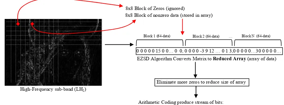
[image:5.595.58.287.239.440.2]8x8 Block of Zeros (ignored)
8x8 Block of nonzero data (stored in array)
0 0 0 0 0 15 0 0… 0 0, 0 0 0 0 -3 9 12 … 0 1 3,0 0 0 0 0…30 0 0 0 0… EZSD Algorithm Converts Matrix to Reduced Array (array of data)
High-Frequency sub-band (LH2)
Eliminate more zeros to reduce size of array
Arithmetic Coding produce stream of bits: 111000010101…etc
[image:6.595.66.523.89.258.2]Block 1 (64-data) Block 2 (64-data) … Block N (64-data)
Figure 6. EZSD algorithm applied on LH2 sub-band.
Reduced Array (67-Data)
Reduced Array (40-Data)
Compressed by Arithmetic Coding to produce new 20 bytes data:
0 0 0 0 0 0 0 0 0 0 0 0 0 0 0 0 0 15 -3 5 9 1 -1 2 -2 -2 0 0 0-3 0 0 0 0-3 0 0 0 012 013 0 0 0 0 0 0 0 030 19 -9 9 8 1 -1 2 -2 0 0 0 0 0 0 0 0
0 8,0 8, 0 1, 15 -3 5 9 1 -1 2 -2 -2 0 3, -3 0 4, -3 0 4, 12 0 1,13 0 8,30 19 -9 9 8 1 -1 2 -2 0 8
[image:6.595.69.520.418.612.2]13 28 132 29 95 29 85 53 114 44 56 37 163 173 191 70 156 213 178 0
Figure 7. Illustrates eliminating more zeros from reduced array.
Already zero position, because it is empty matrix
Compressed stream of data: Arithmetic Decoding produces Reduced Array
13 28 132 29 95 29 85 53 114 44 56 37 ……etc 0 8,0 8, 0 1, 15 -3 5 9 1 -1 2 -2 -2 0 3, -3 0 4, …etc Reconstructed LH2
0 0 0 0 0 15 0 0… 0 0, 0 0 0 0 -3 9 12 … 0 1 3,0 0 0 0 0…30 0 0 0 0…
Expanded Array (i.e. represents original data before convert it to the matrix) Block 1 (64-data) Block 2 (64-data) … Block N (64-data)
Figure 8. Illustrates first phase decoding for LH2 reconstructed.
produced one-dimensional-array contains the original data for the T-Matrix. This array reads element-by- element, and placed in the columns of the T-Matrix.
rows are completes. Figure 9 illustrates DC-Column de- coding.
After generates the T-Matrix, applied Inverse Quanti- zation, It is dot-multiplication of the row coefficients with “Q(n)” (See Equaton (7)), then one-dimensional in-
verse DCT applied on each row to produce 128-values (See Equation (5)), this process will continues until all
3.3. Limited Sequential Search Algorithm Decoding
Figure 9. Second phase for our decompression algorithm “Decoding DC-Column”.
Values. This algorithm is depends on the pointers for finding the missed data inside the Limited-Data for AC- Matrix. If the Limited-Data is missed or destroyed, the AC-Matrix couldn’t return back. Figure 10 shows AC- Matrix decoded by LSS-Algorithm.
The LSS-Algorithm is designed for finding missing data inside a Limited-Data, by using three pointers. These pointers are refers to index in the Limited-Data, the initial value for these pointers are “1” (i.e. first loca-
tion in a Limited-Data). These three pointers are called S1, S2 and S3; these pointers increment by one at each iteration (i.e. these three pointers work as a digital clock,
where S1, S2 and S3 represent hour, minutes and seconds respectively). To illustrate LSS-Algorithm assume we have the following matrix 2 * 3:
EXAMPLE:
30 1 0 19 1 1
In the above example the matrix will compress by us- ing Minimize-Matrix-Size algorithm to produce mini- mized data; M(1) = 3.65 and M(2) = 2.973, the Limited-
Data = {30,19,1,0}. Now the LSS-Algorithm will esti- mates the matrix 2*3 values, by using the Limited-Data and the Random-Weight-Values = {0.1, 0.65, and 0.423}. The first step in our decompression algorithm, assign S1
= S2 = S3 = 1, then compute the result by the following
equation:
3
1
i
Estimated W i Limited S i
(8)W: generated weights. Limited: Limited Data. S(i): pointers 1,2 and 3.
[image:7.595.333.511.86.317.2]LSS-Algorithm computes “Estimated” at each iteration,
Figure 10. Third phase of our decompression algorithm “Decoding AC-Matrix”.
and compare it with “M(i)”. If it is zero, the estimated
values are FOUND at locations= {S1, S2 and S3}. If not
equal to zero, the algorithm will continue to find the ori- ginal values inside the limited-data. The List 3 illustrates LSS-Algorithm, and Figure 11 illustrates LSS-Algorithm estimates matrix values for the above example.
At the fourth phase; our decompression algorithm combines DC-Column and AC-Matrix, and then apply inverse DCT (See Equation (5)) to reconstructs LL2 sub-band, then applying first level inverse DWT on LL2, HL2, LH2 and HH2 to produce approximately LL1. The second level inverse DWT applied on LL1 and other sub- bands are zeros to reconstructs approximately original image.
4. Computer Results
Our compression and decompression algorithm tested on the three gray level images “Lena”, “X-ray” and “Girl”. These images are executed on Microprocessor AMD Athalon ~2.1 GHz with 3G RAM and using MATLAB R2008a programming language under the operating sys- tem Windows-7 (32 bit). Figure 12 shows the three origi- nal images used for test. Our compression algorithm pa- rameters are summarized in the following; 1) Using two level Daubechies DWT “db5”. 2) High-frequencies sub- bands (i.e. HL1, LH1 and HH1) are zeros (ignored). 3) LL2 quantized by Quantization level1 (See Equation (2)) with Quality = 0.005. 4) Applied two dimensional DCT for each 2 × 2 block and Quantization Level2 (See Equa- tion (3)) with R = 5. 5) AC-Matrix compressed by using
Let Limited [1…m]; %% represents Limited Data before process.. Let M [1…p]; % % represents minimized array with size p Let K=3; %% number of estimated coefficients For i=1 to p
S1=1; S2=1; S3=1; %% initial location Iterations=1;
Estimated=W(1)*Limited[S1] + W(2)*Limited[S2]+W(3)*Limited[S3];
While ( (M(i) – Estimated) 0) % check:- if Error =0 or not S3++; % % increment pointer represents "Seconds"
IF (S3>m) S2++; S3=1; end; %% check if S3 is over the limit, return back to "1", and increment S2 IF (S2>m) S1++; S2=1; end;
IF (S1>m) S1=1; end;
Estimated =W(1)*Limited[S1] + W(2)*Limited[S2]+W(3)*Limited[S3]; %% compute Estimated after increments Iterations++; %% compute number of iterations
End; %% end of while
AC_Matrix[i][1]= Limited[S1]; AC_Matrix[i][2]= Limited[S2]; AC_Matrix[i][3]= Limited[S3]; End;
List 3. LSS-Algorithm.
(a)
(b)
[image:8.595.328.519.280.686.2](c)
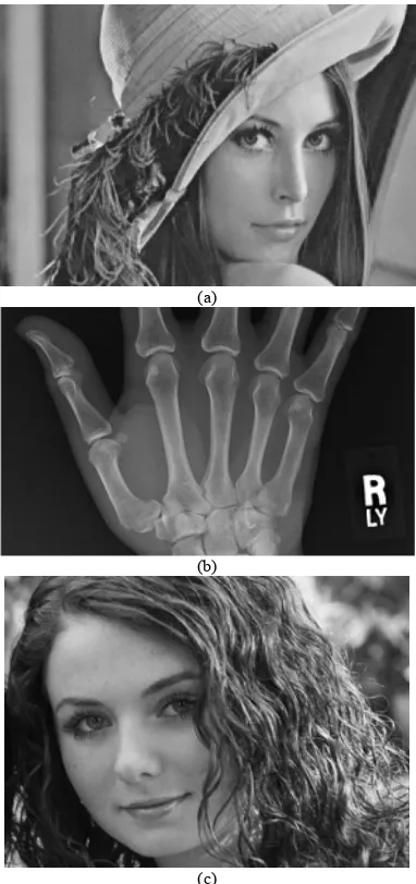
Figure 12. Original images used for test by our approach. (a) Lena image, size = 420 Kbytes, dimension (795 × 539); (b) X-ray image, size = 588 Kbytes, dimension (997 × 602); (c) Girl image, size= 489 Kbytes, dimension (830 × 601).
[image:8.595.105.241.288.706.2]0.423}. 6) High-frequencies (HL2, LH2 and HH2) divided into 8 × 8 blocks, and then compressed by using EZSD algorithm.
Table 1 shows the results of our compression algorithm, for each image with different use of Quality parameter.
Our decompression algorithm illustrated in Section 3, used for decoding the compressed image data, Table 2 shows PSNR for the decoded images and time execution for LSS-Algorithm used to reconstructs AC-Matrix for each image.
PSNR it is used in Table 2, refers to image quality mathematically, PSNR it is a very popular quality mea- sure, can be calculates very easily between the decom-
Table 1. Our compression algorithm results.
Quantization Level1Quality
For quantize high-frequencies sub-bands
HL2, LH2 and HH2
Image Name
Quality = 0.01 Quality = 0.05 Quality = 0.2
Lena Compressed
Size =
25.4 Kbytes 9.8 Kbytes 6.8 Kbytes
X-ray Compressed
Size =
20.2 Kbytes 6.8 Kbytes 5.1 Kbytes
Girl Compressed
Size =
35.5 Kbytes 17.8 Kbytes 10.4 Kbytes
Table 2. PSNR and LSS-Algorithm execution time for de-code images.
PSNR for each Decoded image,
according to Quantization Level1 for
High-Frequencies Decoded
Images
Quality
= 0.01
Quality
= 0.05
Quality
= 0.2
Average Execution
time
Lena 32.9 dB 31.7 dB 30.4 dB 5.9 Sec.
X-ray 37.1 dB 34.9 dB 33.7 dB 3.4 Sec.
Girl 31.5 dB 30.2 dB 27.1 dB 9.7 Sec.
pressed image and its original image [3,4,8]. Our appro- ach is compared with JPEG2000, which is represents one of the best image compression techniques. JPEG2000 consists of; three main phases illustrated in the following steps:
Discrete Wavelet Transform (DWT): Tile components
are decomposed into different decomposition levels us- ing wavelet transform, which improves JPEG2000’s com- pression efficiency due to its good energy compaction and the ability to de-correlate the image across a larger scale [12].
Quantization: In this step, the coefficients obtained
from the wavelet transform are reduced in precision. This process is lossy, unless the coefficients are real and ob- tained by reversible bi-orthogonal 5/3 wavelet transform. The quantizer indices corresponding to the quantized wavelet coefficients in each sub-band are entropy encoded to create the compressed bit-stream. The quantized coef- ficients in a code-block are bit-plane encoded independ- ently from all other code-blocks when creating an em- bedded bit stream [13].
Arithmetic Coding: Arithmetic coding uses a funda-
mentally different approach from Huffman coding in such way that the entire sequence of source symbols is mapped into a single very long codeword. This codeword is built by recursive interval partitioning using the symbol prob- abilities. In this research we used ACDSee applications for save images as JPEG2000 format; an ACDSee appli- cation has many options to save the images as JPEG2000 format. The most option is using; “Quality”. If the image quality is increased the compression ratio is decreased and vice versa. The comparison between JPEG2000 and our approach is based on image quality, when JPEG2000 compressed image size it is equivalent to compressed size by our approach.
Table 3 shows PSNR and compressed size for each image by using JPEG2000 and our approach, and Figure 13, Figure 14 and Figure 15 show decoded images by our approach compared with JPEG2000 according to the quality factor.
Table 3. Comparison between JPEG2000 and our approach.
JPEG2000 Our Approach
Image Name
Quality Compressed Size PSNR Quality Compressed Size PSNR
74% 25.1 Kbytes 35.7 dB 0.01 25.4 Kbytes 32.9 dB
48% 9.83 Kbytes 32.1 dB 0.05 9.8 Kbytes 31.7 dB
Lena
34% 6.81 Kbytes 30.8 dB 0.2 6.8 Kbytes 30.4 dB
61% 20.48 Kbytes 41.6 dB 0.01 20.2 Kbytes 37.1 dB
19% 6.8 Kbytes 36.6 dB 0.05 6.8 Kbytes 34.9 dB
X-ray
2% 5.1 Kbytes 35.6 dB 0.2 5.1 Kbytes 33.9 dB
77% 34.2 Kbytes 33.7 dB 0.01 35.5 Kbytes 31.5 dB
62% 17.8 Kbytes 30.2 dB 0.05 17.8 Kbytes 30.2 dB
Girl
(a) (b) (c)
[image:10.595.64.535.84.306.2]
(d) (e) (f)
Figure 13. Decoded “Lena” image with different quality values by our approach and JPEG2000. (a) Decoded by our ap-proach with Quality = 0.01, PSNR = 32.9 dB; (b) Decoded by JPEG2000 with Quality = 74%, PSNR = 35.7; (c) Decoded by our approach with Quality = 0.05, PSNR = 31.7 dB; (d) Decoded by JPEG2000 with Quality = 48%, PSNR = 32.1 dB; (e) Decoded by our approach with Quality = 0.2, PSNR = 30.4 dB; (f) Decoded by JPEG2000 with Quality = 34%, PSNR = 30.8 dB.
(a) (b) (c)
[image:10.595.77.521.375.571.2]
(d) (e) (f)
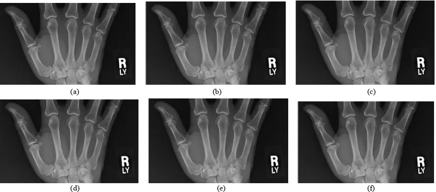
Figure 14. Decoded “X-ray” image with different quality values by our approach and JPEG2000. (a) Decoded by our ap-proach with Quality = 0.01, PSNR = 37.1 dB; (b) Decoded by JPEG2000 with Quality = 61%, PSNR = 41.6 dB; (c) Decoded by our approach with Quality = 0.05, PSNR = 34.9 dB; (d) Decoded by JPEG2000 with Quality = 19%, PSNR = 36.6 dB; (e) Decoded by our approach with Quality = 0.2, PSNR = 33.9 dB; (f) Decoded by JPEG2000 with Quality = 2%, PSNR = 35.6 dB.
[image:11.595.113.484.85.179.2]
(d) (e) (f)
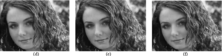
Figure 15. Decoded “Girl” image with different quality values by our approach and JPEG2000. (a) Decoded by our approach with Quality = 0.01, PSNR = 31.5 dB; (b) Decoded by JPEG2000 with Quality = 77%, PSNR = 33.7 dB; (c) Decoded by our approach with Quality = 0.05, PSNR = 30.2 dB; (d) Decoded by JPEG2000 with Quality = 62%, PSNR = 30.2 dB; (e) Decoded by our approach with Quality = 0.2, PSNR = 27.1 dB; (f) Decoded by JPEG2000 with Quality = 46%, PSNR = 28.2 dB.
5. Conclusions
This research introduces a new image compression and decompression algorithms, based on the two important transformations (DCT and DWT) with Minimize-Matrix- Size algorithm and LSS-Algorithm. This research has some advantages illustrated in the following steps:
1) Using two transformations, this helped our com- pression algorithm to increases number of high-fre- quency coefficients, and leads to increases compression ratio.
2) Used two levels quantization for LL2 sub-band and one level quantization for high-frequencies sub-bands at second level DWT. This process increasing number of zeros in the matrix.
3) Minimize-Matrix-Size algorithm it is used to con- verts three coefficients from AC-Matrix, into single flo- ating point value. This process increases compression ratio, and in another hand keep the quality of the high- frequency coefficients.
4) The properties of the Daubechies DWT (db5) helps our approach to obtain higher compression ratio, this is because the high-frequencies for first level is ignored in our approaches. This is because the Daubechies DWT family has the ability to zooming-in, and does not neces- sarily needs for the high-frequencies sub-bands.
5) LSS-Algorithm is represents the core of our decom- pression algorithm, which converts the one-dimensional array into the AC-Matrix. This algorithm is depending on the Random-Weights-Values. LSS-Algorithm finds solu- tion as faster as possible with three pointers (See time execution Table 2).
6) Limited-Data is represents the key of the decom- pressed image, this is represents security for the decom- pressed images, if the users needs to hide the keys.
7) Our approach gives good visual image quality, more than JPEG2000. This is because our approach removes the blurring and an artifact that caused by Multi-level DWT and quantization in JPEG2000 (See Figures 13, 14, 15).
8) The EZSD algorithm used in this research used to removes a lot of zeros, and at same time converts a high-
frequency sub-band to array, this process increases com- pression ratio.
Also this research has some disadvantages illustrated in the following steps:
1) High-frequencies sub-bands at first level of DWT are ignored, this causes low quality decompressed im- ages (See Table 3).
2) The speed of LSS-Algorithm depends on the Limit- Data length for an AC-Matrix; this makes our approach slower than JPEG2000.
3) Minimize-Matrix-Size algorithm converts an AC-Matrix to an array contains stream of floating point va- lues. The minimized array coded by arithmetic coding, the header size of the compressed data may be more than 2 Kbytes.
4) If the Limited-Data for the compressed file is lost or damaged, the image couldn’t be decompressed
REFERENCES
[1] G. Sadashivappa and K. V. S. Ananda Babu, “Performance Analysis of Image Coding Using Wavelets,” IJCSNS International Journal of Computer Science and Network Security, Vol. 8 No. 10, 2008, pp. 144-151.
[2] A. Al-Haj, “Combined DWT-DCT Digital Image Water- marking,” Journal of Computer Science, Vol. 3, No. 9,
2007, pp. 740-746.
[3] K. Sayood, “Introduction to Data Compression,” 2nd Edition, Academic Press, San Diego, 2000.
[4] R. C. Gonzalez and R. E. Woods “Digital Image Proc-essing,” Addison Wesley Publishing Company, Reading, 2001.
[5] M. Tsai and H. Hung, “DCT and DWT Based Image Watermarking Using Sub Sampling,” Proceeding of the Fourth International Conference on Machine Learning and Cybern, Guangzhou, 18-21 August 2005, pp. 5308-
5313.
[6] S. Esakkirajan, T. Veerakumar, V. Senthil Murugan and P. Navaneethan, “Image Compression Using Multiwavelet and Multi-Stage Vector Quantization,” International Jour-nal of SigJour-nal Processing, Vol. 4, No. 4, 2008.
“Image Coding Using Wavelet Transform,” IEEE Trans-actions on Image Processing, Vol. 1, No. 2, 1992, pp. 205-220. doi:10.1109/83.136597
[8] I. E. G. Richardson, “Video Codec Design,” John Wiley & Sons, New York, 2002. doi:10.1002/0470847832 [9] T. Acharya and P. S. Tsai. “JPEG2000 Standard for
Im-age Compression: Concepts, Algorithms and VLSI Ar-chitectures,” John Wiley & Sons, New York, 2005. [10] S. Ktata, K. Ouni and N. Ellouze, “A Novel Compression
Algorithm for Electrocardiogram Signals Based on Wave-let Transform and SPIHT,” International Journal of Sig-nal Processing, Vol. 5, No. 4, 2009, pp. 32-37.
[11] R. Janaki and A. Tamilarasi, “Visually Improved Image Compression by Using Embedded Zero-Tree Wavelet Coding,” IJCSI International Journal of Computer
Sci-ence Issues, Vol. 8, No. 2, 2011, pp. 593-599.
[12] S. M. Basha and B. C. Jinaga, “A Robust Image Com-pression Algorithm Using JPEG 2000 Standard with Golomb Rice Coding,” IJCSNSInternational Journal of Computer Science and Network Security, Vol. 10, No. 12,
2010, pp. 26-33.
[13] C. Christopoulos, J. Askelof and M. Larsson, “Efficient Methods for Encoding Regions of Interest in the Upcom-ing JPEG 2000 Still Image CodUpcom-ing Standard,” IEEE Sig-nal Processing Letters, Vol. 7, No. 9, 2000, pp. 247-249. doi:10.1109/97.863146
[14] M. M. Siddeq, “Image Restoration Using Perception Neural Network,” Master Thesis, Computer Science De-partment, University of Technology, Iraq, 2001.