Combined Eigenfunction Expansion and
Convergence Accelerator Approach to the Rapid
Numerical Evaluation of Hilbert Transforms
Ignacio Porras, Corey D. Schuster, and Frederick W. King
Abstract—The numerical evaluation of a class of Hilbert transforms using an eigenfunction approach is considered. Judicious selection of convergence accelerators allows for the efficient evaluation of the resulting series. The approach is particularly accurate for functions having a Gaussian-like asymptotic behavior. For more slowly decreasing functions, the accuracy of the evaluation decreases.
Index Terms—Hilbert-transform, eigenfunction expansion, convergence accelerators.
I. INTRODUCTION
H
ILBERT transforms occur widely in a variety of prob-lems in science and engineering [1], [2], [3], including applications in the treatment of nonlinear waves, dispersion relations in optical data analysis, and in scattering problems. Gaussian-type functions play a special role in signal analysis, since they are localized in both the time and frequency domains. The construction of the Hilbert transform of many signals such as Gaussian-type pulses is performed in order to cancel negative frequency components, and the transform is most often carried out numerically [2]. An interesting application of the Hilbert transform of Gaussian functions occurs in the analysis of the heat equation [4]. As a consequence in part, the numerical evaluation of Hilbert transforms has been studied intensely using a number of different approaches [3], [5], [6], [7], [8], [9], [10], [11].The Hilbert transform of a function f, denoted Hf, is defined by
(Hf) (x) = 1 πP
Z ∞
−∞ f(s)
x−sds, (1)
where P designates the Cauchy principal value, which can be expressed as
(Hf) (x) = 1 πǫlim→0+
Z x−ǫ
−∞ f(s) x−sds+
Z ∞
x+ǫ
f(s) x−sds
.
(2) The Hilbert transform is also defined using the opposite sign convention to that given in Eq. (1).H is a linear operator fromLp(R)→Lp(R), for1< p <∞[3], [13], [14], where
Manuscript received March 27, 2011; revised April 15, 2011. Support from the National Science Foundation, the Donors of the Petroleum Re-search Fund, administered by the American Chemistry Society, and the Office of University Research, University of Wisconsin-Eau Claire, are greatly appreciated. We also thank the Spanish Ministerio de Educaci´on, which provided financial assistance for the visit of I. Porras (PR2007-0456), who also acknowledges funding from project FPA2009-14091-C02-02.
I. Porras: Departmento de F´ısica At´omica, Molecular y Nuclear, Univer-sidad de Granada, E-18071 Granada, Spain. C.D. Schuster and F.W. King: Depatment of Chemistry, University of Wisconsin-Eau Claire, Eau Claire, Wisconsin 54702
Lp(R) denotes the Banach space of Lebesgue integrable
functions:
Lp(R) =
f :R→C,
Z ∞
−∞
|f(x)|pdx <∞
. (3)
The most important case occurs for the Hilbert space
L2(R). If f(x) is an even function, f(−x) = f(x), then Eq. (1) can be expressed as
(Hf) (x) =2x π P
Z ∞
−∞ f(s)
x2−s2ds, (4)
and iff(x)is an odd function,f(−x) =−f(x), then
(Hf) (x) = 2 πP
Z ∞
−∞ sf(s)
x2−s2 ds, (5)
Equations (4,5) are often referred to as the Kramers-Kronig transforms of even and odd functions, respectively.
A comment on notation is appropriate: (Hf(s))(x) in-dicates the Hilbert transform off evaluated at the pointx, andsis the dummy integration variable. This is written more concisely as(Hf)(x), when there is no need to specify the integration variable. If there is no risk of confusion, we will writeH[f(x)]for the Hilbert transform when the functional form is specified.
There is continuing interest in the development of accurate numerical methods for the evaluation of Hilbert transforms and other related singular integrals [6], [7], [8], [9], [10], [11], [15], [16], [17], [18], [19]. There is also an extensive body of work devoted to the numerical determination of the Kramers-Kronig transforms [16].
Weideman [17] studied the numerical evaluation of the Hilbert transform of a functionf ∈L2(R)using an expan-sion technique in terms of the eigenfunctions of the Hilbert transform operator, which can be written as:
ϕn(x) =
(1 +ix)n
(1−ix)n+1 , for n∈Z. (6) Weideman examined several examples, for which he ob-tained the coefficientsbn. For the case f(x) = 1/(1 +x2),
the results are exact, since the function can be expanded in a compact closed form in terms of the eigenfunctions in Eq. (6). For functions that decay in a significantly different manner from this example, the eigenfunction decomposition approach of Weideman yielded more slowly convergent series.
II. THEORY
Two similar methods are presented here for the numerical evaluation of the Hilbert transform in terms of a numerical series.
In our first approach, the Hilbert transform is expressed in terms of an expansion of Hermite functions, which are eigenfunctions of the Fourier transform operator. We start by expanding our function of interest (assumed of L2(R)) as
f(x) = ∞ X
n=0
αnun(x), (7)
whereun(x)are the orthonormal Hermite functions, defined
in terms of the standard Hermite polynomialsHn(x)by:
un(x) =p 1
2nn!√πHn(x)e
−x2
/2, (8) and the coefficientsαn are determined from:
αn =
Z ∞
−∞
f(x)un(x)dx. (9)
An analysis of convergence issues associated with the expansion in Eq. (7) can be found in the work of Boyd [20].
We define the operator
T =sgnxF, (10)
where sgnxdenotes the signum function:
sgnx=
1 , x >0 0 , x= 0 −1 , x <0
, (11)
and F stands for the Fourier transform operator, a unitary operator onL2(R). It is obvious thatT is a linear isometric (bounded) operator onL2(R), therefore it is continuous. The action of T on the function f(x) can be also expanded in the same basis set:
Tf(x) = ∞ X
m=0
µmum(x), (12)
where the coefficientsµm can be expressed as:
µm=
Z ∞
−∞
sgnx(Ff)(x)um(x)dx. (13)
ApplyingT to Eq. (7), it follows that:
sgnx(Ff)(x) = ∞ X
n=0
αnsgnx(Fun)(x), (14)
where we have used the fact thatT is linear and continuous. The basis functionsun(x)satisfy [21]:
(Fun)(x) = (−i)nun(x) (15)
and
(F−1u
n)(x) =inun(x). (16)
Employing Eq. (15) allows Eq. (14) to be simplified to
sgnx(Ff)(x) =sgnx ∞ X
n=0
αn(−i)nun(x). (17)
On substituting Eq. (17) into Eq. (13) leads to the follow-ing result for the coefficientsµm:
µm=
∞ X
n=0
αn(−i)n
Z ∞
−∞
sgnx um(x)un(x)dx, (18)
which can be rearranged, using the property un(−x) =
(−1)nun(x), to yield
µm=
∞ X
n=0
αn(−i)n1−(−1)n+m
Z ∞
0
um(x)un(x)dx.
(19) The non-vanishing terms in the previous sum are those for whichn+m is odd. Let m= 2k andn= 2j+ 1, for any
k, j non-negative integers, then
µ2k =−i
∞ X
j=0
α2j+1(−1)jIk,j (20)
and ifm= 2k+ 1 andn= 2j, then
µ2k+1= ∞ X
j=0
α2j(−i)jIj,k, (21)
whereIk,j is defined by
Ik,j= 2
Z ∞
0
u2k(x)u2j+1(x)dx. (22) Using the key connection between the Fourier and Hilbert transforms [3], [13], [14],
(FHf)(x) =−isgnx(Ff)(x), (23)
it follows from Eq. (12) and employing Eq. (16), that
(Hf)(x) = −iF−1 ∞ X
m=0
µmum(y)
!
(x)
= −i ∞ X
m=0
µmimum(x). (24)
Rewriting Eq. (24) to account for the even and odd contributions ofmand substituting Eqs. (20) and (21), leads to the final result:
(Hf)(x) = − ∞ X
k=0
(−1)ku2k(x)
∞ X
j=0
(−1)jα2j+1Ik,j
+ ∞ X
k=0 (−1)ku
2k+1(x) ∞ X
j=0 (−1)jα
2jIj,k. (25)
TheIk,j integral can be evaluated from Eq. (22) by using a
relationship between Hermite polynomials and the associated Laguerre polynomialsL(jα)(x), and employing the change of
variablet=x2, to obtain
Ik,j =
(−1)k+j2k+j+1/2k!j!
p
(2k)!(2j+ 1)!π Z ∞
0
L(k−1/2)(t)L
(1/2)
j (t)e
−tdt.
(26) The integral in Eq. (26) can be solved in terms of the gamma function Γ(z), by writing both polynomials as a series inL(0)m and then employing the orthogonality relation
for Laguerre polynomials, to yield
Z ∞
0
L(−1/2)
k (t)L
(1/2)
j (t)e
−tdt
= 2Γ k+
1 2
Γ j+32
π(2j−2k+ 1)Γ(k+ 1)Γ(j+ 1), (27)
so that
Ik,j =
(−1)k+j2k+j+3/2Γ k+1 2
Γ j+32 π3/2(2j−2k+ 1)p
The preceeding formula can be expressed in terms of double factorials as
Ik,j = (−1)
k+j√2(2k−1)!!(2j+ 1)!!
(2j−2k+ 1)p
π(2k)!(2j+ 1)!. (29)
Equation (25) reflects the fact that the Hilbert transform of an even function is an odd function and vice versa. When the functionf(x) is even or odd, the right-hand side reduces to only one double sum because everyα2k+1orα2k,
respectively, is zero. Furthermore, for functions for which all
αm are zero for m greater than a finite value, the second
summation of both terms is a finite sum.
The second numerical approach investigated involves ap-plying the Hilbert transform directly to Eq. (7), to obtain
(Hf)(x) = ∞ X
n=0
αnH[un(x)]. (30)
where we have made use of the fact thatH is a continuous operator onL2(R). Therefore, the right-hand side converges in the norm sense. If we expand explicitly the Hermite polynomials, we can write:
(Hf)(x) = 1 π1/4
∞ X
n=0 2np
(2n)!α2nχ(1)n
+ √
2 π1/4
∞ X
n=0
2np(2n+ 1)!α2n+1χ(2)n (31)
where
χ(1)
n = n
X
m=0
(−1)mHhx2(n−m)e−x2
/2i
4mm!(2n−2m)! (32)
and
χ(2)n = n
X
m=0
(−1)mHhx2(n−m)+1e−x2
/2i
4mm!(2n−2m+ 1)! . (33)
The Hilbert transforms H[x2(n−m)e−x2
/2] and
H[x2(n−m)+1e−x2/2
] can be reduced in closed form to the function H[e−x2
/2], and the latter can be evaluated [3] as:
H[e−x2/2
] =−ie−x2/2
erf(ix/√2), (34)
where erf(z)denotes the error function, defined by ([22], p. 297)
erf(z) = √2 π
Z z
0
e−t2
dt. (35)
One of the strengths of this approach occurs when the function of interest can be expanded in a finite series using Eq. (7), then the Hilbert transform can be computed accu-rately. Only one infinite series is encountered for a general function of interest, not taking into account the particular evaluation strategy forHhxke−x2
/2i, whereas in the Fourier transform approach, two infinite series will be encountered in many cases.
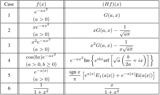
TABLE I
EXACTHILBERT TRANSFORMS FOR THE FUNCTIONS INVESTIGATED NUMERICALLY.
Case f(x) (Hf)(x)
1 e
−ax2
(a >0) G(a, x)
2 xe
−ax2
(a >0) xG(a, x)− 1
√aπ
3 x
2e−ax2
(a >0) x
2G(a, x)
−x√1aπ
4 cos(bx)e −ax2
(a >0, b≥0) e
−ax2 Im
n
eibxerfh√a b 2a+ix
io
5 e
−a|x|
(a >0)
sgnx π
ea|x|E
1(a|x|) +e−a|x|Ei(a|x|)
6 1
1 +x2
x
1 +x2
III. COMPUTATIONALAPPROACH
For the numerical evaluation of the Hilbert transform we have selected the test functions displayed in Table I. These functions show a range of different asymptotic decays and their Hilbert transforms can be evaluated analytically, and therefore provide useful test cases for numerical comparison. For notational compactness G(a, x) is used to denote the Hilbert transform H[e−ax2
/2], for a > 0, and can be expressed as
G(a, x) =−ie−ax2
erf(i√ax). (36)
The special functions appearing in Table I are the expo-nential integral functions, defined by (see for example [22], p. 228)
Ei(z) =−P Z ∞
−z
e−t
t dt, (37)
and
E1(z) =
Z ∞
1
e−zt
t dt, (38)
and Im denotes the imaginary part.
[image:3.595.303.559.88.240.2]For the test functions employed, the corresponding expan-sion coefficientsαn obtained from Eq. (9) are tabulated in
Table II. In these cases, they can be evaluated in closed form, which is an obvious advantage for the application of our method, and we will use them in the computations reported. However, this approach does not require that the expansion coefficients be known explicitely, as they can be determined numerically by Gauss-Hermite quadrature or other numerical integration methods in a straightforward manner. In this table,Γ(a, z)denotes the incomplete gamma function and 1F1(a;b;z) designates the Kummer confluent hypergeometric function.
It is obvious that if the function has a well defined parity, only non-zero coefficients with either an even or odd index arise.
We note parenthetically that it is easy to find examples where the αm expansion coefficients can be determined
analytically, but the Hilbert transform cannot be evaluated in a simple closed form, for example:
f(x) = log|x|e−ax2
TABLE II
EXPANSION COEFFICIENTS OF DIFFERENT TEST FUNCTIONS.
f(x) Expansion coefficientsα2norα2n+1
x2me−ax2
(a >0) α2n=
p
(2n)!√π
22m+n a+1 2
n+m+12 n X
j=0
(−1)j(2m+ 2n−2j)! a+1 2
j
j!(m+n−j)!(2n−2j)!
x2m+1e−ax2
(a >0) α2n+1=
p
(2n+ 1)!√π
22m+n+32 a+1
2
n+m+32 n X
j=0
(−1)j(2m+ 2n+ 2−2j)! a+1 2
j
j!(m+n+ 1−j)!(2n+ 1−2j)!
cos(bx)e−ax2
(a >0, b≥0) α2n=
p
(2n)!√π
2n a+1 2
n+12 n X
j=0
(−1)j a+1 2
j
1F1
1
2−j+n; 1 2;
−b2
2(1+2a)
j!(n−j)!
e−a|x|
(a >0)
α2n =
22n+12p(2n)!
π1/4
n X
j=0
(−1)j 8jj!(2n−2j)!
Γn−j+1 2
1F1
n−j+1 2;
1 2;
a2
2
− √2aΓ(n−j+ 1)1F1
n−j+ 1;3 2;
a2
2
1
1 +x2 α2n=
p
(2n)! e√π
2n n X
j=0
(−1)jΓ j−n+1 2,12
j!(n−j)!
The present approach is demonstrated by first considering the simple example
f(x) =x2me−x2
/2. (40) Since this function is even, it can be expanded using Eq. (7) only containing terms with even indexes. Thus, Eq. (25) simplifies to:
(Hf)(x) = ∞ X
k=0
(−1)ku2k+1(x)
m
X
j=0
(−1)jα2jIj,k. (41)
Let us consider the particular test case m = 1, then the expansion coefficients are α0 = π1/4/2, α2 = π1/4/21/2,
α2n= 0 forn >1, and hence
(Hf)(x) = r√
π 2
∞ X
k=0
(−1)k√2I0,k−I1,k
u2k+1(x). (42) As a second example, consider
f(x) =x2m+1e−x2
/2. (43) In an analogous fashion, the expansion coefficients can be found, and Eq. (25) simplifies to
(Hf)(x) =− ∞ X
k=0
(−1)ku2k(x) m
X
j=0
(−1)jα2j+1Ik,j. (44)
In the two preceeding examples, the functions can be written as a finite series using Eq. (7), and the resulting Hilbert transform contains a single infinite series.
A slightly more generalized example is the following function wherea >0, anda6= 1/2,
f(x) =x2me−ax2
, (45)
and the expansion coefficients are displayed in Table II. The resulting Hilbert transform now involves two infinite series. However, it should be noted that a rescaling of the expansion variable leads to the inner series expansion being a finite sum, which yields a more efficient numerical approach.
That is, the Hilbert transform can be evaluated using
(Hf)(x) = 1
2a m
Hht2me−t2
/2i √2ax, (46) and the expansion in Eq. (41).
For the preceding examples in Eqs. (40), (43) and (45), the Hilbert transform can be found in terms of a single infi-nite series, which is most effectively evaluated by applying convergence acceleration techniques, when direct summation is too inaccurate. We now focus on the general case where a finite series for Eq. (7) cannot be obtained, resulting in a double infinite series. To apply a convergence accelerator to the general case we make use of an interchange of order of summation [23] for Eq. (25), transforming the double infinite series to a combination of finite and infinite series of the form:
(Hf)(x) = − ∞ X
k=0 (−1)k
k
X
j=0
α2j+1Ik−j,ju2(k−j)(x)
+ ∞ X
k=0 (−1)k
k
X
j=0
α2jIj,k−ju2(k−j)+1(x).(47)
Five different convergence accelerators were tested: these were the Levin-u [24] and Levin-t′
[25], [26] transforma-tions, the Weniger-1 and Weniger-2 [26], [27], [28] transfor-mations, and the Wynnǫ-algorithm [29], [30].
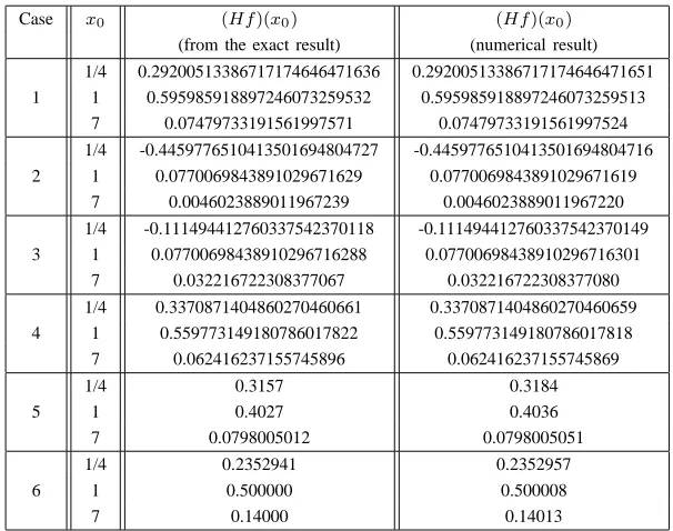
IV. RESULTS ANDDISCUSSION
Using the exact formulas from Table I we were able to test the numerical evaluations for the two different approaches. A comparison of the numerical results obtained using Eq. (31), with the exact evaluations of the Hilbert transform for the test functions is shown in Table III.
The test functions 1-4 gave the best results, with the number of significant digits decreasing as the value of
x increased. These four test functions exhibit a Gaussian behaviour similar to the Hermite functionsun(x)and hence
TABLE III
ACOMPARISON OF NUMERICAL VALUES FOR THEHILBERT TRANSFORM VERSUS THE EXACT EVALUATION FOR THE TEST FUNCTIONS GIVEN IN TABLEI. THE VALUESa= 12/11ANDb= 11/13HAVE BEEN EMPLOYED.
Case x0 (Hf)(x0) (Hf)(x0)
(from the exact result) (numerical result) 1/4 0.29200513386717174646471636 0.29200513386717174646471651 1 1 0.595985918897246073259532 0.595985918897246073259513
7 0.07479733191561997571 0.07479733191561997524 1/4 -0.4459776510413501694804727 -0.4459776510413501694804716 2 1 0.0770069843891029671629 0.0770069843891029671619
7 0.0046023889011967239 0.0046023889011967220 1/4 -0.111494412760337542370118 -0.111494412760337542370149 3 1 0.07700698438910296716288 0.07700698438910296716301
7 0.032216722308377067 0.032216722308377080 1/4 0.3370871404860270460661 0.3370871404860270460659 4 1 0.559773149180786017822 0.559773149180786017818
7 0.062416237155745896 0.062416237155745869
1/4 0.3157 0.3184
5 1 0.4027 0.4036
7 0.0798005012 0.0798005051
1/4 0.2352941 0.2352957
6 1 0.500000 0.500008
7 0.14000 0.14013
functions have an asymptotic decay that closely matches a Gaussian function, and as a result the expansion coefficients converge much more slowly. By examining either Eq. (31) or Eq. (47), we see that the only difference between the numerical Hilbert transform of two different functions is the expansion coefficients associated with that function. This indicates a direct correlation between the behaviour of the expansion coefficients and the rate of convergence of the Hilbert transform.
For functions with a Gaussian character, the expansion of the present work will improve on the accuracy obtained using the expansion of Weideman [17]. This is expected because of the choice of basis functions for the expansion. As we move to functions exhibiting slower rates of asymptotic decay, the expansion of Weideman will lead to higher accuracy. For example, for cases like f(x) =x2e−ax2
,a >0, the present approach gives a very compact closed form expansion, which can be evaluated with high efficiency. Here the present approach is significantly better in both computational speed and accuracy compared with the Weideman approach, whilst for a case likef(x) = (1 +x2)−1we encounter the opposite situation, where the latter technique leads to a closed form solution with only two terms, and the approaches described in this work would require much more computational ef-fort. For cases including some oscillatory behaviour, for example, working with f(x) = (cosx + sinx)e−x2
or
f(x) = 2+sincosxxe−x2
, we have found that the computational speed of both approaches is similar, but the accuracy is better with the approach of the present work.
With respect to the performance of the convergence accel-erators employed in this work, the best results were obtained using the Wynn ǫ-algorithm. On writing the general result, given by Eq. (47), in the form:
(Hf)(x) = ∞ X
k=0
[image:5.595.146.449.88.327.2]ak(x), (48)
Fig. 1. Plot of the individual terms ak(x) for the Hilbert transform calculated from Eq. (48) for case 4 withx= 1.
and analyzing the individual termsak(x)for case 4 withx=
1, the sequence behaved in a non-monotonic manner with irregular signs, as shown in Fig. 1. This would be somewhat similar to the terms generated from the functionsin(kx)/k. For this situation, Wynn’s algorithm is expected to be the most suitable choice for convergence acceleration [31].
The Levin and Weniger convergence accelerators offered satisfactory accuracy, but less compared to the Wynn ǫ -algorithm. Based on the form of the series, the performance of this method is not surprising [31]. Table IV shows a com-parison of the convergence accelerators employed using the test functionf(x) = cos(bx)e−ax2
and employing Eq. (47). The other test functions exhibited similar trends in the relative precision for the different convergence accelerators investigated, so the results in Table IV are representative of the observed trends.
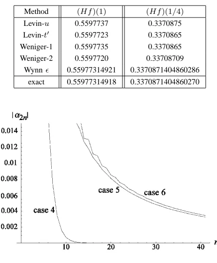
TABLE IV
ACOMPARISON OF THE DIFFERENT CONVERGENCE ACCELERATOR METHODS USING THE FUNCTIONf(x) = cos(bx)e−ax2
. THE VALUES
a= 12/11ANDb= 11/13HAVE BEEN EMPLOYED.
Method (Hf)(1) (Hf)(1/4) Levin-u 0.5597737 0.3370875 Levin-t′ 0.5597723 0.3370865 Weniger-1 0.5597735 0.3370865 Weniger-2 0.5597720 0.33708709
[image:6.595.59.277.94.358.2]Wynnǫ 0.55977314921 0.3370871404860286 exact 0.55977314918 0.3370871404860270
Fig. 2. Comparison of the expansion coefficients for cases 4, 5, and 6.
for the test functions employed, we indeed see a trend in their convergence rates as mentioned previously. To keep Fig. 2 uncluttered, only the expansion coefficients for cases 4-6 are shown. The convergence rate for case 4 is slower than for cases 1-3, but we see from Fig. 2 that the convergence rate of case 4 is much faster than either case 5 or case 6. The results in Fig. 2 provide support for the rate of convergence of the expansion coefficients in either Eq. (31) or Eq. (47) being an important factor, as expected, in determining ac-curate numerical values for the Hilbert transform. The other important factor in determining accurate results is the optimal selection of convergence accelerator to apply. The numerical method proposed by Weideman also showed that a slower convergence rate for the expansion coefficients resulted in a slower converging Hilbert transform.
The Fourier transform method offered a few more digits of precision over the direct series method forx= 1/4. For
x= 1both methods performed equally well and forx= 7
the direct method offered a few more digits of precision over the Fourier method.
V. CONCLUSION
Two methods have been presented for the numerical evaluation of the Hilbert transform, both of which are com-putationally efficient, and both yield accurate results for a number of test functions. The approaches are particularly effective for functions exhibiting a Gaussian-like asymptotic behavior. Five different convergence accelerator techniques were employed to sum the series that arise, with the Wynn
ǫ-algorithm providing the best accuracy for this particular application.
REFERENCES
[1] S. L. Hahn, Hilbert transforms in Signal Processing, Boston: Artech House, 1996.
[2] S. L. Hahn, in The Transforms and Applications Handbook, A.D. Poularikas, ed., CRC Press (Boca Raton, 1996), p. 463.
[3] F. W. King, Hilbert Transforms, Cambridge University Press (Cam-bridge, 2009).
[4] E. Kochneff, Y. Sagher, and K. Zhou, Homogeneous solutions of the heat equation, J. Approx. Theory 69, (1992) 35-47.
[5] R. Kress and E. Martensen, Anwendung der Rechteckregel auf die relle Hilberttransformation mit unendlichem intervall, Zeit. Ang. Math. Mech. 50, (1970) T61-T64.
[6] S. J. Collocott, Numerical solution of Kramers-Kronig transforms by a Fourier method, Comput. Phys. Commun. 13, (1977) 203-206. [7] S. J. Collocott and G. J. Troup, Adaptation: numerical solution of the
Kramers-Kronig transforms by trapezoidal summation as compared to a Fourier method, Comput. Phys. Commun. 17, (1979) 393-395. [8] O. E. Taurian, A method and a program for the numerical evaluation of
the Hilbert transform of a real function, Comput. Phys. Commun. 20, (1980) 291-307.
[9] G. A. Gazonas, The numerical evaluation of Cauchy principal value integrals via the fast Fourier transform, Int. J. Computer Math. 18, (1986) 277-288.
[10] B. D. Vecchia, Two new formulas for the numerical evaluation of the Hilbert transform, BIT 34, (1994) 346-360.
[11] K. Diethelm, A method for the practical evaluation of the Hilbert transform on the real line, J. Comput. Appl. Math. 112, (1999) 45-53. [12] R. Afshar, F. M. Mueller, and J. C. Shaffer, Hilbert transformation of densities of states using Hermite functions, J. Comput. Phys. 11, (1973) 190-209.
[13] P. L. Butzer and R. J. Nessel, Fourier Analysis and Approximation,
Volume 1 One-Dimensional Theory, Academic Press, (New York, 1971).
[14] J. N. Pandey, The Hilbert Transform of Schwartz Distributions and
Applications, John Wiley and Sons, (New York, 1996).
[15] F. W. King, G. J. Smethells, G. T. Helleloid, and P. J. Pelzl, Nu-merical evaluation of Hilbert transforms for oscillatory functions: A convergence accelerator approach, Comput. Phys. Commun. 145, (2002) 256-266.
[16] F. W. King, Efficient numerical approach to the evaluation of Kramers-Kronig transforms, J. Opt. Soc. Am. B 19, (2002) 2427-2436. [17] J. A. C. Weideman, Computing the Hilbert transform on the real line,
Math. Comp. 64, (1995) 745-762.
[18] K. Diethelm, Peano kernels and bounds for the error constants of Gaussian and related quadrature rules for Cauchy principal value integrals, Numer. Math. 73, (1996) 53-63.
[19] K. Diethelm, New error bounds for modified quadrature formulas for Cauchy principal value integrals, J. Comput. Appl. Math. 82, (1997) 93-104.
[20] J. P. Boyd, The rate of convergence of Hermite function series, Math. Comp. 35, (1980) 1309-1316.
[21] H. Hochstadt, Integral Equations, John Wiley and Sons, (New York, 1973), p. 146-148.
[22] M. Abramowitz and I. A. Stegun (eds.), Handbook of Mathematical
Functions, Dover, (New York, 1964), p. 775.
[23] E. R. Hansen, A Table of Series and Products, Prentice-Hall, (New Jersey, 1975), p. 14.
[24] D. Levin, Development of non-linear transformations for improving convergence of sequences, Int. J. Comput. Math. 3, (1973) 371-388. [25] D. A. Smith and W. F. Ford, Acceleration of linear and logarithmic
convergence, SIAM J. Numer. Anal. 16, (1979) 223-240.
[26] E. J. Weniger, Nonlinear sequence transformations for the acceleration of convergence and the summation of divergent series, Comput. Phys. Rep. 10, (1989) 189-371.
[27] E. J. Weniger, On the derivation of iterated sequence transformations for the acceleration of convergence and the summation of divergent series, Comput. Phys. Commun. 64, (1991) 19-45.
[28] E. J. Weniger, Nonlinear sequence transformations: A computational tool for quantum mechanical and quantum chemical calculations, Int. J. Quantum Chem. 57, (1996) 265-280; Erratum: Int. J. Quantum Chem. 58, (1996) 319-321.
[29] J. Wimp, Sequence Transformations and Their Applications, Academic Press, (New York, 1981).
[30] P. Wynn, On a procrustean technique for the numerical transformation of slowly convergent sequences and series, Proc. Cambridge Philos. Soc. 52, (1955) 663-671.