Data Clustering and Topology Preservation Using 3D Visualization of Self Organizing Maps

Data Clustering and Topology Preservation Using 3D

Visualization of Self Organizing Maps

Z. Mohd Zin, M. Khalid, E. Mesbahi and R. Yusof

Abstract— The Self Organizing Maps (SOM) is regarded as an

excellent computational tool that can be used in data mining and data exploration processes. The SOM usually create a set of prototype vectors representing the data set and carries out a topology preserving projection from high-dimensional input space onto a low-dimensional grid such as two-dimensional (2D) regular grid or 2D map. The 2D-SOM technique can be effectively utilized to visualize and explore the properties of the data. This technique has been applied in numerous application areas such as in pattern recognition, robotics, bioinformatics and also life sciences including clustering complex gene expression patterns. In this paper, the structure of traditionally 2D-SOM map has been enhanced to a three-dimensional Self Organizing Maps (3D-SOM) maps. It has the purpose to directly cluster data into 3D-SOM space instead of 2D-SOM data clusters. The primary works mostly involved the extensions of SOM algorithm in particular the number, relation and structure arrangement of its output neurons, neighbourhood weight update processes and distances calculation in 3D xyz-axis. The proposed method has been demonstrated by computing 3D-SOM visualization on iris flowers dataset using high level computer language. The performance of 2D-SOM and 3D-SOM in terms of their quantization errors, topographic errors and computational time has been investigated and discussed. The experimental results have shown that the 3D-SOM has been able to form a 3D data representation, has slightly higher quantization error and computational time but performed better topology preservation than in 2D-SOM.

Index Terms— 3D Self Organizing Maps, Neural Network, Data

Clustering, Iris flowers, quantization error, topographic error

I. INTRODUCTION

lustering is the task of organizing a set of objects into meaningful groups or clusters which can be disjoint, overlapping or organized in some hierarchical fashion. As described in (1), the key element of clustering is the notion that the discovered groups are meaningful. In some applications, it could be said that the similarity between the objects in the same groups could be maximized while the similarity between objects of different groups could be minimized in order for a cluster to be meaningful. In other word, an object can be described either by a set of measurements or relationships between objects in the same or different groups (2).

Manuscript received March 13, 2012.

Zalhan Mohd Zin is a lecturer with Universiti Kuala Lumpur Malaysia France Institute, 43650 Bandar Baru Bangi, Selangor, Malaysia. (phone: +603-8926-2022; fax: +603-8925-8845; e-mail: [email protected],edu.my).

Marzuki Khalid is a professor with Universiti Teknologi Malaysia, Kuala Lumpur, Malaysia. (email: [email protected]).

Ehsan Mesbahi is a professor with Newcastle University, United Kingdom (e-mail: [email protected]).

Rubiyah Yusof is a professor with Universiti Teknologi Malaysia, Kuala Lumpur, Malaysia. (email: [email protected]).

Furthermore, clustering can also be considered as an exploratory tool for analyzing large data sets and has been used extensively in numerous application such as in the area of pattern recognition, robotics, bioinformatics and also life sciences (1) including clustering complex gene expression patterns (3) (4) (5) (6) (7). Besides that, the SOM has also been found very useful for the study of ecological communities and sciences. In (8), the authors have shown that the SOM is useful and has comparable performance with other ordination techniques for the study of ecological modelling. A comprehensive study of SOM technique that has been applied to various ecological sciences problems has been addressed in (9).

In fact, the limitations of the 2D-SOM when dealing with high dimensionality and complex data such as gene expression data have been highlighted in a review done in (4). The authors have presented a survey on various gene expression clustering techniques that have been used including SOM. They have also indicated that too few output neurons in the SOM gives large within-cluster distance, and too many output neurons will results in meaningless data diffusion. In their case, the sizes of dimension only vary in 2D xy-axis. In (6), the authors have described that higher-dimensional map is possible, but it would be difficult to visualize and it is not commonly used. In the work done in (3), the authors have indicated some difficulties that are associated with U-matrix, a method to visualize the SOM as described in (10), for a highly-dimensional input data when the dimension of SOM is small. They have introduced a side intensity modulated SOM (SIM-SOM) method that provides distinct line of separation between clusters when dealing with this U-matrix limitation. In the recent comprehensive review on SOM application to ecological science (9), the authors have suggested that the development of the SOM could be also based on its network architecture, convergence in complex spatial and temporal data, and the adaptability to evolve toward more efficient and sophisticated SOM in order to deal with the complexity in ecological processes. Therefore, advancement in visualization technique of SOM has also been expected to be further researched and studied.

introduced it for their music archive but this design was limited to only 3x3x3 SOM map. On the other hand, by using primary colour elements, the 3D-SOM topology was also found to be more informative and had revealed differences between geo-referenced elements that were not usually accessible with the application of 2D SOM (14). Meanwhile in (16), by using the toolbox in (12), the authors had improved the U-matrix and neurons arrangements to 3D-SOM structure for data clustering, but the performance of this structure was not evaluated.

Therefore, in this research, the focus was given to enhance the technique of traditional 2D-SOM map by proposing a 3D-SOM output visualization to cluster the data. The proposed technique should be able to form clustered data representation in 3D axis. The purpose of this 3D-SOM visualization would be to provide much bigger clustering space ability along the third axis, z-axis, without extending the dimensions of SOM along its traditional xy-axis. The primary work of the research involved the development of a 2D-SOM and later a 3D-SOM computer program using high level computer language. The comparison of the performance of quantization and topographic errors for clustering iris flowers between 2D-SOM and 3D-2D-SOM has been done through experimental works.

II. METHODS

A. The 2D Self Organizing Maps (2D-SOM)

The SOM or Kohonen Map is an unsupervised artificial neural network technique and was developed by Teuvo Kohonen (17). It creates a set of prototype vectors representing the data set and carries out a topology preserving projection of the prototypes from high-dimensional input space onto a low-dimensional grid such as 1D or 2D grid of map units. This artificial neural network training involves the process of adjusting weights of neurons to the distributions of the input data. After the training process has been performed, clusters are identified by mapping object to the output neurons. As mentioned in (5), the SOM can be interpreted as a topology preserving mapping from input space onto the 2D grid map units. The elements of the SOM display can be called output neurons, map units or even virtual units, term that has been used in (8) for ecological modelling. The number of output neurons which typically varies from a few dozen up to several thousand usually determines the accuracy and generalization capability of the SOM. The SOM is trained iteratively and as described in (8) (17), the SOM algorithm can be presented in six following steps:

 Step-1: Epoch t=0, the output neurons , ∈

{1, . . , }, ∈{1, . . , } are initialized with random values ℎ ∈{0, . . ,1}.

 Step-2: A sample vector , ∈{1, . . , } is randomly chosen from the input data set. n is the number of items or species.

 Step-3: Using Euclidean distance method, the distances between and all the output neurons ℎ ∈

{1, . . , }, ∈{1, . . , } are computed.

 Step-4: Choose the winning neuron or the Best-Matching-Unit (BMU), which is denoted by . It is the

output neuron with prototype closest to as described in equation eq-1:

− = − (eq-1)

 Step-5: The output neurons are updated. The BMU/ and its topological neighbours are moved closer to the input vector in the input space. The update rule for the output neuron is as in equation eq-2:

( + 1) = ( ) + ( )ℎ ( )[ − ( )]

(eq-2)

where is time, ( ) is adaptation coefficient or learning rate and ℎ is a neighbourhood kernel function that centred on the winner unit:

ℎ ( ) = exp −

( ) (eq-3)

 Step-6: Increase time t to t+1. If ( < ) then go to Step-2 else stop the training.

In eq-3, and are positions of neurons and on

the SOM grid. − is the Euclidean distance between two points on the map between winning unit and each output neurons . Both ( ) and ( ) decrease monotonically with time. The neighbourhood function in eq-3 is a Gaussian function and it is the commonly used neighbourhood function in SOM. The intensity of the updating process is controlled by neighbourhood function, ℎ , which is focused to the winner neuron that having closest reference vector, . Once the SOM training has been completed, the computed distances between the input data vectors and the updated weights are calculated and the data are then mapped into their respective output neurons.

B. The 3D Self Organizing Maps(3D-SOM)

The focus of the research was on the development of 3D-SOM, an enhanced SOM visualization technique that should be able to cluster data in three-dimensional xyz-axis. The 3D-SOM program has been developed by using high level computer language. In this work, the same training algorithm of SOM as in (17) (8) has been applied. The six steps of 2D-SOM mentioned previously have been programmed and extended later to handle 3D-SOM visualization. Figure 1 shows the proposed technique consist multiple 2D 3x3 neurons layers that have been stacked one on top of each other along z-axis layer.

Fig. 1: The 3D-SOM 3x3x3 output neurons’ positions viewed from the top of z-axis.

The number of prototype vectors or weights was equalled to the number of output neurons, v. All these weights were associated between the input neurons and the output neurons. The overview of the relations between the input vectors, weights and output neurons in 3D-SOM is shown in Figure 2. The weights were initialized in the same manner as in Step-1 of the 2D-SOM previously. In Step-2, a sample vector

, ∈{1, . . , } is randomly chosen from the input data set. In iris flowers dataset experiment, this sample vector was selected from its n species. In the next step, Step-3, the distances between and all the output neurons were computed. This selection of BMU, denoted by , was done using the following equation:

− = − (eq-5)

where i, j and k represent the indexes of x, y and z-axis respectively. After the selection of the winning neuron, the next major step of 3D-SOM was to update the topological neighbours of this BMU by using equation eq-2, eq-3 and Gaussian function. The weights update process in 3D-SOM

has been done in similar way as in SOM algorithm but this time this process has occurred in 3D xyz-axis.

Fig. 2: Relation between the input vectors, reference vectors and output neurons in 3D-SOM.

In fact, in 3D-SOM, the possible positions of BMU neighbours has increased drastically due to the existence of the third axis, z-axis. The neighbours’ positions with respect to x-axis, y-x-axis, z-x-axis, xy-x-axis, xz-x-axis, yz-axis or xyz-axis now had to be taken into considerations. An example is that a neuron that is located at the most top left edge in 2D-SOM has only three adjacent neuron neighbours while a neuron with similar position in the 3D-SOM has seven adjacent neighbours. Figure 3 show an example of selected BMU positions with its adjacent and non-adjacent neighbours in 2D-SOM and 3D-2D-SOM In 3D-2D-SOM and in eq-3 in particular, , the position of neuron could also be located in the z-axis in addition to xy-axis. Therefore, the value of − which was considered as the distance between two output neurons in three-dimensional xyz-axis. At the end of 3D-SOM training, the computed distances between the input data vectors and the updated weights were calculated. Finally, the data were then mapped into their respective output neurons based on the closest distance between both of them.

C. Performance measurement of SOM

One of the benefits of SOM is its ability to preserve the topology in the projection (20). The performance of SOM is usually analyzed by using two common criteria which are the quantization error, qe and topographic error, te. Both of them have been used to verify the quality of the SOM in (12). The first criterion represents the value of resolution while the second criterion represents the topology preservation.

According to (20), qe is equaled to the average distance between each data vector and it’s best matching unit (BMU) after SOM training. It can also be defined as following equation:

qe = ∑ ⃗ − ⃗ (eq-7)

where N is the number of data vectors and _⃗ is the best matching prototype of the corresponding ⃗ data vector. The smaller the quantization error indicates the closer data vectors mapped to its closest output neurons. Meanwhile, the topographic error, te, measures the proportion of all data vectors for which first and second BMUs are not adjacent units, and it can be defined as follow:

te = ∑ ( )⃗ (eq-8)

The topographic error is calculated as in (eq-8) where the function ( ⃗) is 1 if ⃗ data vector’s first and second BMUs are not adjacent and 0 otherwise. These standard qe and te as in (eq-7) and (eq-8) have been used to observe the performance of 3D-SOM compared to 2D-SOM in clustering iris flowers dataset in this research.

III. EXPERIMENTAL FRAMEWORKS AND RESULTS

The experiments for both 2D-SOM and 3D-SOM have been conducted with same parameters and the initial values and increasing number of output neurons in each x, y and z-axis. For these experimental works purposes, the 2D-SOM and 3D-SOM algorithms have been trained using sequential learning. The initial weights have been randomly initialized between 0 and 1. For both techniques, in rough phase, the learning rate, α used was 0.5 and decreased linearly to zero while in fine-tuning phase, the learning rate used was 0.05 and also decreased linearly to zero. The neighbourhood functions used were Gaussian function. The number of iterations has been set to 2000 for rough phase and 80000 for fine tuning phase. The experiments were conducted using Intel Core2Quad 2.5 GHz with 2.0 Gb memory. The iris flowers dataset consist of 150 flowers and they are divided into three equal numbers (50) that represents three different classes of flowers, Setosa, Versicolor and Virginica. This dataset can be obtained in (21). In each flower, four features

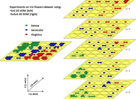
were measured in cm, the length and width of sepal; and the length and width of petal. With varied dimensions from 4x4 until 7x7 output neurons, the classes of Setosa and Virginica flowers have been appropriately clustered far from each others, while the class of Versicolor flower has been clustered between these two classes, and closer to Virginica class. This distribution of iris flowers species was consistent with the nature of the iris flowers dataset itself where Setosa class is linearly separable from the other two classes, and these two other classes are not linearly separable from each other as described in (21).

For comparison, the result of iris flowers dataset clustering using 5x5 2D-SOM and 5x5x5 3D-SOM is shown in Figure 4. In 3D-SOM, the z-axis represents five different layers where each layer has 25 output neurons. In this figure too, the Virginica class has dominated mostly the two topmost layers while Setosa class has dominated mostly the two most bottom layers. Furthermore, Versicolor seems to be quite evenly distributed in all layers and they have maintained their locations in the middle between Setosa and Virginica classes throughout the five layers. There were also no appearances of Setosa classes in the two topmost layers. Only Versicolor and Virginica classes have appeared on them which could be interpreted that the dissimilarity between Setosa and Virginica has been shown by 3D-SOM throughout its z-axis. It also seems that the 3D-SOM has provided more output neurons or in other word, more space for the data to be clustered vertically.

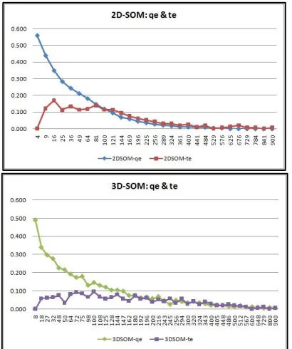
On the other hand, a number of experimentation works have also been performed to observe the performance of 2D-SOM and 3D-2D-SOM techniques when clustering iris dataset. There were 30 experiments of 2D-SOM with the total number of output neurons started from 4(2x2) until 900(30x30). Meanwhile, in 3D-SOM case, 43 experiments have been conducted with the total number of output neurons started from 8(2x2x2) until also 900(10x10x9). The number of output neurons in x, y and z-axis has varied from small to large in all experiments. The quantization and topographic errors measurement as described in the previous section have been applied. For each experiment in 2D-SOM and 3D-SOM, the program was run five times and the average values of both errors were taken. Their results are shown in Figure 5.

In this figure, the values of quantization error and topographic error have been plotted according to the number of output neurons used in both techniques. In 2D-SOM case, the average time taken was between 0.5 seconds for 4 units and 49.42 seconds for 900 units while it took between 1.02 seconds for 8 units and 50.35 seconds for 900 units in 3D-SOM. This indicates that the computational time increased when the number of output neurons increased for both 2D-SOM and 3D-2D-SOM techniques. Furthermore, the time taken was slightly larger in 3D-SOM than in 2D-SOM because the number of adjacent neighbours is higher in 3D-SOM as described in Figure 3.

Fig. 5: The quantization errors and topographic errors obtained in 2D-SOM (top) and 3D-SOM(bottom). Horizontal axis represents the total number of output neurons while vertical axis represents the error.

From the results in Figure 5 too, the quantization errors and topographic errors in 3D-SOM behaved the similar way with those in 2D-SOM. It seems that as in 2D-SOM, the higher number of output neurons has also contributed to the lower values of quantization and topographic errors in 3D-SOM. The results have shown consistent error behaviours as in (20) where the authors mentioned that when the number of units increased there were more neurons to represent the data, and each data vector will be then closer to its BMU. In our case, the proposed 3D-SOM structure has also shown the same behaviour as 2D-SOM structure in terms of these quantization and topographic errors. Therefore, the technique of 3D-SOM could be said as having comparable performance as in 2D-SOM for data clustering. The main difference between these two techniques lies on the visualization approach of data-neuron mapping where 2D-SOM map data on its 2D map while 3D-SOM map data on its 3D space. It was also noticed that 3D-SOM training consumed higher computational time due to its larger number of adjacent neighbour’s calculation.

IV. CONCLUSIONS

The SOM is considered as one of the excellent computational tools for data clustering. It can cluster data and map them into the usual 2D map. In this paper, the technique of 2D-SOM has been developed and programmed using high level computer language of C/C++ and later it has been enhanced to a 3D-SOM visualization technique for the purpose of clustering data in 3D xyz-axis instead of data clustering in traditional 2D-SOM xy-axis output map. The works have mainly involved in developing the technique, algorithm, output neuron arrangements and also C/C++ program. The major tasks taken were mostly involved the Step-3, Step-4, Step-5 and Step-6 of the SOM algorithm as described in Section 2. These steps were crucial as they represent very important elements of SOM algorithm which involved the structure of SOM’s output neurons and its neighbourhood weights updates. From the experimental results, both 2D-SOM and the 3D-SOM have been able to cluster iris flowers dataset according to their respective classes of Setosa, Virginica and Versicolor. The 3D-SOM visualization technique was also able to cluster data using its xyz-axis output neuron’s arrangement or structure. Besides that, the results have also shown that the 3D-SOM had slightly higher quantization error and computational time but performed better topology preservation than in 2D-SOM. The technique could also be used for clustering data that might not be obviously clustered neither easily interpreted using the traditional 2D-SOM such as the data that could be in very large size, high complexity and has multidimensional properties. Additional research could be undertaken to apply and analyze the 3D-SOM technique for clustering other complicated type of data such as gene expression data. Finally, the 3D-SOM visualization technique has the potential to be considered as another alternative pattern classifier visualization technique and could also be implemented in other suitable applications.

REFERENCES

[1] Zhao, Ying and Karypis, George. Clustering in Life Science.

Methods in Molecular Biology. New Jersey : Humana Press Incorporation, 2007, Vol. 224, pp. 183-218.

[2] Jain, Anil K. and Dubes, Richard C. Algorithm for Clustering Data. New Jersey : Prentice Hall Incorporation, 1998.

[3] A New SOM-based Visualization Technique for DNA Microarray Data. Jagdish C. Patra, Ee Luang Ang, Pramod K. Meher,

Qin Zhen. Vancouver, Canada : s.n., 2006. International Joint Conference on Neural Networks.

[4] Techniques for Clustering Gene Expressions Data. Kerr, G., et

al. 3, s.l. : Elsevier Incorporation, 2008, Computers in Biology and Medecine, Vol. 38, pp. 283-293.

[5] Analysis and Visualization of Gene Expression Microarray Data in Human Cancer Using Self-Organizing Maps. Sampsa

Hautaniemi, Olli Yli-Harja,Jaakko Astola,Päivikki Kauraniemi,Anne Kallioniemi,Maija Wolf,Jimmy Ruiz,Spyro Mousses & Olli-P. Kallioniemi. 2003, Journal of Machine Learning, Vol. 52, pp. 45-66.

[6] A Modified Kohonen Network for DNA Splice Junction Classification. Thanakorn Naenna, Robert A Bress, Mark J

Embrechts. Chiang Mai, Thailand : s.n., 2004. IEEE Region Ten Conference on Analog and Digital Techniques in Electrical Engineering . pp. 215-218.

[7] Self Organizing Maps for Cluster Analysis of A Breas Cancer Database. Mia K. Markey, Joseph Y. Lo,Georgia D.

[8] A Comparison of Self Organizing Map Algorithm and Some Conventional Statistical Methods for Ecological Community Ordination. J. L. Giraudel, S. Lek. s.l. : Elsevier, 2001, Journal of Ecological Modelling, Vol. 146, pp. 329-339.

[9] Self Organizing Maps Applied to Ecological Sciences. Chon,

Tae-Soo. 1, s.l. : ScienceDirect, 2011, Ecological Informatics, Vol. 6, pp. 50-61.

[10] A Nonlinear Projection Method Based on Kohonen's Topology Preserving Maps. Martin A. Kraaijveld, Jianchang Mao,Anil

K. Jain. 1995. IEEE Transaction on Neural Networks. pp. 548-559.

[11] Clustering of the Self Organizing Maps. Juha Vesanto, Esa

Alhoniemi. 3, 2000, IEEE Transaction on Neural Networks, Vol. 11, pp. 586-600.

[12] Juha Vesanto, Johan Himberg, Esa Alhoniemi & Juha Parhankangas. SOM Toolbox for Matlab 5. 2000. p. 59, Technical report.

[13] Design of a Structured 3D SOM as a Music Archive. Arnulfo

Azcarraga, Sean Manalili. Espoo, Finland : Springer, 2011. International Workshop on self Organizing Maps. Vol. 6731, pp. 188-197.

[14] Jorge Gorrichaa, Victor Loboa. Improvements on the visualization of clusters in geo-referenced data using Self-Organizing Maps. Computers and Geosciences. s.l. : Elsevier, 2011, Vol. 37.

[15] Position Detection of Unexploded Ordnance from Airborne Magnetic Anomaly Data Using 3-D Self Organized Feature Map (3D SOFM). TarekEl Tobely, Ahmed Salem. 2005. IEEE Symposium on Signal Processing and Information Technology.

[16] A Consideration on the multi-dimensional topology in Self-Organizing Maps. Kikuo Fujimura Kazuhiro Masuda, Yutaka

Fukui. Totori, Japan : s.n., 2006. International Symposium on Intelligent Signal Processing and Intelligent System (ISPACS). [17] The Self-Organizing Maps. Kohonen, Teuvo. s.l. : IEEE Xplore,

1990. Proceedings of the IEEE. Vol. 78, pp. 1464-1480. [18] Haykin, S. Neural Networks, a Comprehensive Foundations.

s.l. : Prentice Hall, 1999.

[19] On the Use of Self Organizing Maps for Clustering and Visualization. Flexer, Arthur. Prague, Czech Republic : Springerlink, 1999. International Conference on Principle on Data Mining and Knowledge Discovery. Vol. 5, pp. 80-88. [20] Topology Preservation in SOM. E. Arsuaga Uriaite, F. Diaz

Martin. 1, 2005, International Journal of Mathematical and Computer Sciences, Vol. 1, pp. 19-22.

[21] Fisher, R. A. UCI Machine Learning Repository. Center for Machine Learning and Intelligent System University of California Irvine. [Online] 2006. [Cited: January 31, 2011.] Iris Database. http://archive.ics.uci.edu/ml/datasets/Iris.

[22] Vesanto, Juha. SOMToolbox Homepage. Laboratory of Computer and Information Science (CIS) Helsinki Universiti of Technology. [Online] 2008. [Cited: January 20, 2011.] http://www.cis.hut.fi/somtoolbox/.

[23] Self Organizing Maps for Cluster Analysis of A Breast Cancer Database. Mia K. Markey, Joseph Y. Lo,Georgia D.