Abstract—This paper studies three statistical downscaling methods to predict temperature and rainfall at 45 weather stations in Thailand. Methods under consideration are multiple linear regressions (MLR), support vector machine with polynomial kernel (SVM-POL), and support vector machine with Radial Basis Function kernel (SVM-RBF). Large-scale data are from Geophysical Fluid Dynamics Laboratory (GFDL). Five predictor variables are chosen: (1) temperature, (2) pressure, (3) precipitation, (4) evaporator, and (5) net short wave. Accuracy is assessed by 10-fold cross-validation in terms of root-mean-squared error (RMSE) and correlation coefficient (R). SVM-RBF is the most accurate model. Prediction accuracy of monthly average rainfall and temperature is satisfying in most part of the country. Lastly, downscaling models can project long term trends of monthly average rainfall and temperature.
Index Terms— statistical downscaling, temperature, rainfall, multiple linear regressions, support vector machine.
I. INTRODUCTION
eneral Circulation Models (GCMs) are widely accepted as a tool for predicting future climate change. However, output from GCMs cannot be used for local prediction directly because GCMs operate in large scale. It is necessary to bring output from GCMs down to small scale for local prediction. Downscaling is a method to derive local climate information from relative GCM output.
Two downscaling approaches that are commonly used are statistical downscaling and dynamical downscaling. Statistical downscaling assumes that relationships between large scale and local climate are constant. It combines GCM output with local observations in order to obtain their statistical relationships. Local climate forecast can then be determined from such relationships. Dynamical downscaling involves nesting regional climate model into an existing global climate model. Numerical meteorological modeling is used in dynamical downscaling approach.
Various methods have been employed to derive relationships in statistical downscaling to forecast different climate information in different parts of the world. Such
Manuscript received December 28, 2010 ; revised January 22, 2011 Miss Pawanrat Aksornsingchai is a master's degree student in the school of Computer Engineering Faculty of Engineering at King Mongkut's Institute of Technology, Ladkrabang, Chalongkrung Rd., Ladkrabang, Bangkok, Thailand, Postal code:10520, (e-mail: [email protected]).
Asst. Prof. Dr. Chutimet Srinilta was with the school of Computer Engineering Faculty of Engineering at King Mongkut's Institute of Technology, Ladkrabang, Chalongkrung Rd., Ladkrabang, Bangkok, Thailand, Postal code:10520 Phone number +66(0) 2329 8000 - 2329 8099; (e-mail: [email protected], [email protected]).
methods include canonical correlation analysis, multiple linear regressions, artificial neural networks and support vector machine. The rest of this section summarizes some previous studies on statistical downscaling methods.
Katrin Maak et al. [6] discussed statistical downscaling with canonical correlation analysis to validate the flowering date of Galanthus nivalis L. at 74 stations in Northern Germany. Observation period was in January, February and March of the years 1890 to 1990. They found a strong linear correlation between flowering dates and monthly mean near-surface air temperatures. Statistical model was built from twenty years of observed data. The prediction was accurate. In addition, they paid extra attention to scenarios when atmospheric CO2 concentration increased. It was
found that air temperature alone was a sufficient predictor when CO2 concentration was doubled and tripled.
Huth [7] evaluated several statistical downscaling models and predictors in estimating daily mean temperatures during winter at 39 stations in central Europe. Data from eight winter seasons (December 1982-February 1983 to December 1989-February 1990) were used in the study. Downscaling methods under consideration were canonical correlation analysis, singular value decomposition analysis, and three multiple regression models (full regression, stepwise regression and pointwise regression). Chosen predictors were 500 hPa heights, sea level pressure, 850 hPa temperature and 1000–500 hPa thickness. Pointwise regression outperformed other methods. The best predictor for daily mean temperature at regional average and individual station levels was the combination of heights and temperature. Temperature alone gave more accurate estimate than circulation variables.
Dibike et al. [11] compared two downscaling models— temporal neural network (TNN) model and regression-based statistical model. Models were to predict daily precipitation, daily minimum temperature and daily maximum temperature in northern Quebec, Canada. Six combinations of 6-7 predictors were evaluated. Thirty years of data (1961-1990) were used to construct the models. Seasonal model biases were discussed. It was found that the TNN model was more efficient in downscaling both daily precipitation and daily maximum and minimum temperatures.
Tripathi et al. [10] proposed the support vector machine (SVM) approach for statistical downscaling to obtain average monthly rainfall at meteorological sub-divisions (MSDs) in the entire India. The period of study extended from January 1948 to December 2002. The SVM model was compared against multilayer back-propagation neural network based model. They concluded that SVM based
Statistical Downscaling for Rainfall and
Temperature Prediction in Thailand
Pawanrat Aksornsingchai and Chutimet Srinilta
model was a suitable statistical downscaling method for precipitation.
Hua Chen et al. [4] compared three downscaling models—relevance vector machine (RVM), least square support vector machine (LSSVM) and back propagation neural network (BPNN). The focus of the study was on the effect of climate change on runoff change of Danjiang Kou reservoir, China. Time period was from 1960 to 2000. They also tried to simulate future scenario prediction. They found that the RVM model was an effective way to assess climate change impact on hydrology.
The following objectives have been set for our study. Firstly, to see the effect of grid size on model accuracy, secondly to evaluate three statistical downscaling methods in estimating monthly average rainfall and temperature at weather stations in Thailand, and lastly, to see the trend of monthly average rainfall and temperature in the next four years.
The paper is organized as follows. Section II introduces statistical downscaling process and three downscaling methods that were used in experiments. Section III describes data that were used to construct and test models. Model accuracy measures are explained in Section IV. Section V discusses three sets of experiments. Section VI concludes the paper.
II.STATISTICAL DOWNSCALING TECHNIQUES A.Statistical downscaling process
Statistical downscaling is based on an assumption that there is a strong relationship between large-scale predictor(s) and small-scale predictand. Predictor(s) can be used to determine predictand when they co-vary with similar time structure.
Common GCM predictor choices include geopotential heights and sea surface temperature. According to [3], the frequently used predictors to predict temperature and rainfall are sea level pressure, height, temperature, and the relative humidity. Common predictands are temperature and rainfall at a local weather station. Statistical model determines values of predictand from predictor.
B.Multiple linear regressions
Multiple linear regression (MLR) is a statistic method that is used to model a linear relationship between a dependent variable (predictand) and one or more independent variables (predictors). MLR is a least square-based method. Predictand is a continuous variable. MLR assumes that the relationship between variables is linear. Therefore, the MLR model can be expressed as a linear function shown in Equation 1.
n n
x
x
x
y
=
β
1 1+
β
2 2+
...
+
β
, (1) wherey
is the value of a predictand, xiis the value of the ith predictor variable, and βiis an adjustable error coefficient of the ith predictor variable.Multiple linear regression attempts to find a best fit plane. The fit can be evaluated by the coefficient of multiple determination (R2). The correlation coefficient (R) expresses the degree to which two or more predictors are related to the predictand.
C.Support vector machine
Support vector machines (SVMs) are a set of related supervised learning methods that are used in classification and regression analysis. Basic idea of the SVM for regression analysis is explained below.
Consider the finite training sample pattern
(
xi,yi)
, where Ni R
x∈ is a sample value of the input vector x consisting of N training patterns (i.e.,x=x1,...,xN) and yi∈R is the corresponding value of the desired model output. A non-linear transformation function is defined to map the input space to a higher dimension feature space, Rh
A non-linear relation between inputs and outputs in the original input space are shown in Equation 2.
b x w x f
yˆ= ( )= TΦ( )+ , (2) where
y
ˆ
is the actual model output,w and
b
are adjustable coefficients model parameters.The objective function in support vector machines task is
2 min
2 w
w
subject to yi
(
w⋅xi+b)
≥1,i=1,2,...,N (3) The constrained may derive from dual Lagrangian is) ( ) ( 2 1 , 1 j i j i j j i i n i i
D yy x x
L =
∑
−∑
Φ ⋅Φ=
λ λ
λ (4)
Because it’s very difficult to computation involve calculating transformed vector, the solution method called kernel trick.The mapping kernel can be defined as
( )
x,y (x) (y)K =Φ ⋅Φ (5) The kernel trick is a method for calculating similarity in the transformed space using the original space, helps to address in mapping function by Mercer’s Theorem, computing time using kernel function is cheaper than using the transformed attribute set, avoided curse of dimensionality problem because the computations are performed in the original space.
Mercer’s Theorem is a function to perform mapping of the attributes of the original space to the feature space.
{
( ), ( )}
) ,
(x x x x
K ′ =
φ
φ
′ (6) A polynomial kernel mapping is a popular method for non-linear modeling.{ }
dx x x x
K( , ′)= , ′ (7)
{ }
{
}
dx x x x
K( , ′)= , ′ +1 (8) Radial Basis Function (RBF) kernel is used to map the input data into higher dimensional feature space, which is given by ⎟ ⎟ ⎠ ⎞ ⎜ ⎜ ⎝ ⎛ − ′ − = ′ 2 2 2 exp ) , ( σ x x x x
K , (9)
where
σ
is the width of RBF kernel which can be adjusted to control the expressivity of RBF. The RBF kernels have localized and finite responses across the entire range of predictors.III. DATA A.GFDL data
We used Geophysical Fluid Dynamics Laboratory (GFDL CM2.x) reanalyzed data (2.25°lat.x3.75°long, scenarios A2 and B2) in our experiments. Five predictors were chosen: (1) surface (skin) temperature (TSTAR in oK); (2) surface pressure (PSTAR in 2
dynes/cm ); (3) precipitation (rain + snow: PRECIP in cm/day); (4) evaporation (EVAPOR in cm/day); and (5) net short wave at the top (SWTOP in
2 /m
W ).
GFDL CM2.x scenarios A2 and B2 were chosen for the experiments. “The A2 family of scenarios is characterized by, a world of independently operating, self-reliant nations, continuously increasing population, regionally oriented economic development, slower and more fragmented technological changes and improvements to per capita income. The B2 scenarios are of a world more divided, but more ecologically friendly. The B2 scenarios are characterized by, continuously increasing population, but at a slower rate than in A2, emphasis on local rather than global solutions to economic, social and environmental stability, intermediate levels of economic development, less rapid and more fragmented technological change than in A1 and B1” [1, 3].
B.Observed data
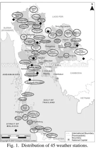
Region of study was the country Thailand (5ºN–22ºN latitudes and 95ºE–105ºE longitudes). We used local weather data from Thai Meteorological Department. Rainfall and temperature were collected from 45 weather stations located at every part of the country. Provinces where 45 weather stations were situated are circled in Figure 1.
The observation period spanned from January 1965 to September 2007.
Thailand is covered by 96 (12x8) GFDL grid points. IV. MODEL ACCURACY MEASURES
Data were divided into 2 groups. The first group (was used to train model, and the second group was used to test model. 10-fold cross validation was used to assess the accuracy of model. Accuracy measures were root-mean-squared error (RMSE), correlation coefficient (R), mean absolute error (MAE), relative absolute error (RAE), and root relative squared error (RRSE).
V.EXPERIMENTS A.Set 1 : Grid size
The purpose of this set of experiments was to see the effect of GFDL grid sizes to model accuracy.
A support vector machine model with Radial Basis Function kernel (SVM-RBF) was used.
[image:3.595.346.509.47.298.2]Three different GFDL grid sizes— 1x1, 3x3, 5x5 were examined.
Fig. 1. Distribution of 45 weather stations.
Results
Table I shows rainfall and temperature prediction accuracy of the model at Bangkok station when grid size was varied.
TABLEI
MODEL ACCURACY WITH DIFFERENT GRID SIZES
(BANGKOK STATION,SVM-RBFMODEL) Predictand/
Scenarios Grid Size
R MAE RMSE RAE
(%)
RRSE (%) 1x1 0.6219 2.3782 3.5223 69.36 82.36
rain / A2 3x3 0.6467 2.2725 3.3481 66.28 78.29 5x5 0.6869 2.1583 3.1999 62.95 74.82 1x1 0.5913 2.4771 3.6786 72.25 86.02
rain / B2 3x3 0.6038 2.3991 3.5182 69.97 82.27 5x5 0.6644 2.2343 3.2776 65.17 76.64 1x1 0.7907 0.6787 0.9340 63.70 65.42
temp / A2 3x3 0.8307 0.6052 0.8067 56.80 56.50 5x5 0.8396 0.5854 0.7831 54.94 54.85 1x1 0.7854 0.7063 0.9663 66.29 67.68
temp / B2 3x3 0.8300 0.5992 0.8098 56.23 56.72 5x5 0.8390 0.5802 0.7816 54.45 54.74
We can see from Table I that when 5x5 grid was chosen, the model gave the most accurate output (MAE, RMSE, RAE, RRSE values were the lowest and R is closest to 1) at Bangkok station in both scenarios.
In addition, we also tested at other 44 weather stations and found that the results could be interpreted in the same direction—5x5 GFDL grid gave the highest accuracy. Due to space limitation, we could not present accuracy measures at other weather stations.
Grid size was fixed at 5x5 in all other sets of experiments. B.Set 2 : Statistical downscaling methods
The purpose of this set of experiments was to evaluate three statistical downscaling methods: (1) multiple linear regression (MLR); (2) support vector machine with polynomial kernel (SVM-POL), and (3) support vector machine with Radial Basis Function kernel (SVM-RBF).
grid points and Hua Chen et. al [4] used 24 grid points in their experiments.
Accuracy of monthly average of all 45 stations from the three downscaling methods was measured in terms of RMSE and R. In addition, we took a closer look at Bangkok weather station by finding four accuracy measures at the station.
Results
Table II shows accuracy of three downscaling methods under consideration.
TABLEII
ACCURACY OF DOWNSCALING MODELS
(ALL 45STATIONS) Predictand /
Scenarios
RMSE R
MLR SVM
-POL
SVM
-RBF
MLR SVM
-POL
SVM
-RBF
rain / A2 3.41 2.89 2.83 0.64 0.72 0.74
rain / B2 3.50 2.96 2.88 0.62 0.70 0.72
temp / A2 1.11 0.92 0.88 0.81 0.86 0.88
temp / B2 1.01 0.92 0.88 0.81 0.86 0.87
The lowest RMSE values of rainfall and temperature predictands were 2.83 and 0.88, respectively. Both were resulted from SVM-RBF model. In addition, values of R from SVM-RBF model were closest to 1 in both rainfall and temperature predictands. Thus, SVM-RBF model gave the most accurate monthly average rainfall and temperature in all 45 weather stations.
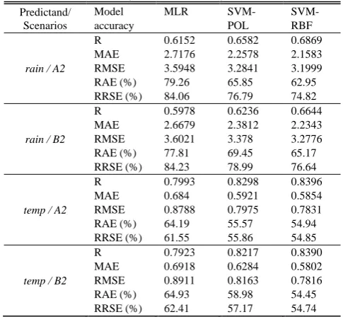
Table III expresses model accuracy comparison using all four accuracy measures.
TABLEIII
ACCURACY OF DOWNSCALING MODELS
(BANGKOK STATION) Predictand/
Scenarios
Model accuracy
MLR SVM- POL
SVM- RBF
R 0.6152 0.6582 0.6869
MAE 2.7176 2.2578 2.1583
rain / A2 RMSE 3.5948 3.2841 3.1999
RAE (%) 79.26 65.85 62.95 RRSE (%) 84.06 76.79 74.82
R 0.5978 0.6236 0.6644
MAE 2.6679 2.3812 2.2343
rain / B2 RMSE 3.6021 3.378 3.2776
RAE (%) 77.81 69.45 65.17 RRSE (%) 84.23 78.99 76.64
R 0.7993 0.8298 0.8396
MAE 0.684 0.5921 0.5854
temp / A2 RMSE 0.8788 0.7975 0.7831
RAE (%) 64.19 55.57 54.94 RRSE (%) 61.55 55.86 54.85
R 0.7923 0.8217 0.8390
MAE 0.6918 0.6284 0.5802
temp / B2 RMSE 0.8911 0.8163 0.7816
RAE (%) 64.93 58.98 54.45 RRSE (%) 62.41 57.17 54.74
The focus was at Bangkok weather station. The two SVM based models outperformed the MLR based model in all predictand-scenario combinations. The four measures all agreed.
For temperature predictand, the SVM-RBF model was superior in both scenarios. For rainfall predictand, the SVM-RBF model performed better in scenario A2 and the SVM-POL model was better in scenario B2.
SVM-RBF downscaling method was used in all experiments in Sets 3 and 4.
C.Set 3 : Prediction
The purpose of this set of experiments was to find prediction accuracy of the model (SVM-RBF).
Three weather stations were chosen from each of the four regions of Thailand—northern, north eastern, central and southern. Locations of these 12 weather stations are marked with diamonds in Figure 1.
Predictands were monthly average rainfall and temperature at these 12 weather stations from the year 1991 to the year 2007.
Results
Table IV shows RMSEvalues of monthly average rainfall and temperature predictands in both scenarios. Prediction accuracy of temperature was higher than that of rainfall at all 12 stations under both scenarios.
TABLEIV
PREDICTION ACCURACY (RMSE) MONTHLY AVERAGE RAINFALL AND TEMPERATURE
(12STATIONS,1991-2007) Weather
station Region
rain A2
rain B2
temp A2
temp B2 Maehongson northern 1.9232 1.9988 1.1183 1.0435 Nan northern 2.5218 2.4070 1.0938 1.0297 Phitsanulok northern 2.7308 2.5118 0.9623 0.8855 Loei northeastern 2.3352 2.2483 1.1058 1.0139 Mukdahan northeastern 2.6490 2.6449 1.4168 1.3310 Ubon
Ratchathani northeastern 2.4722 2.7118 1.1126 1.1126 Chainat central 2.1962 2.1066 0.8774 0.8225 Suphanburi central 2.3676 2.2564 1.0340 0.9262 Bangkok central 3.2050 2.9762 1.0712 0.9979 Phetchaburi southern 2.5214 2.5201 0.7044 0.6872 Phuket southern 3.2043 3.4266 0.9159 0.9259 Narathiwat southern 6.0269 5.7578 0.6070 0.6123
We took a closer look at four weather stations in four regions from 2005-2007. Selected stations were Maehongson station (northern region), Loei station (northeastern region), Bangkok station (central) and Phetchaburi station (south region).
Actual observed and predicted monthly average rainfall values are shown in Figures 2-5. Predicted rainfall values from both scenarios were very close, especially in northern and northeastern regions. The observed and predicted rainfall values varied in the same direction at all four stations. Predicted rainfall values were quite close to actual rainfall values observed at northern station most of the time. The observed values were much higher than the predicted values only 1-2 times each year when it rained the most. We could say the same to station in the northeastern region. However, prediction accuracy was lower at central and southern stations.
[image:4.595.44.287.443.667.2]lower at central station.
Fig. 2. Monthly average rainfall Maehongson station (northern region)
Fig. 3. Monthly average rainfall Loei station (northeastern region)
Fig. 4. Monthly average rainfall Bangkok station (central region)
[image:5.595.46.551.41.724.2]Fig. 5. Monthly average rainfall Phetchaburi station (southern region)
Fig. 6. Monthly average temperature Maehongson station (northern region)
Fig. 7. Monthly average temperature Loei station (northeastern region)
Fig. 8. Monthly average temperature Bangkok station (central region)
Fig. 9. Monthly average temperature Phetchaburi station (southern region)
D.Set 4 : Future prediction
were very close to actual observed. Model was constructed from SVM-RBF downscaling methods. From experiment set 3, scenario B2 resulted in lower RMSE in both rainfall and temperature prediction in northeastern region. Therefore, we chose scenario B2 for this set of experiments.
Results
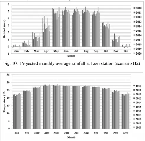
The projected rainfall and temperature values at Loei station are shown in Figures 10 and 11.
The most rainy months are May(2010, 2011 and 2019), June(2016), July(2013, 2015, 2017), August(2012, 2014, 2020), and September (2018). The least rainy months are January(2010, 2011, 2014-2018, 2020) and December (2012, 2013, 2019).
[image:6.595.47.293.288.526.2]Projected average temperature in any given month does not vary much throughout the ten-year period. Highest temperature occurs in April(2012, 2013, 2017-2019) and May(2010, 2011, 2014-2016, 2020). Lowest temperature occurs in January(2010, 2012-2016, 2018, 2020), and December (2011, 2017, 2019).
Fig. 10. Projected monthly average rainfall at Loei station (scenario B2)
Fig. 11. Projected monthly average temperature Loei station (scenario B2)
VI. CONCLUSION
Four sets of experiments were conducted in our study. The first set was about GFDL grid size. It was found that 5x5 grid yielded the highest model accuracy. Therefore, it was used in all other sets of experiments together with five predictors (TSTAR, PSTAR, PRECIP, EVAPOR and SWTOP) and two scenarios (A2 and B2). In the second set of experiments, one MLR based and two SVM based (SVM-POL and SVM-RBF) statistical downscaling methods were evaluated in terms of ability to forecast rainfall and temperature at 45 weather stations Thailand. Observation period was from January 1965 to September 2007. The SVM-RBF model was the most accurate model among the three. The third set of experiments determined prediction accuracy at selected weather stations from every part of Thailand. Focused period was 2005-2007. In general, observed values and predicted values varied in similar manner. However, temperature prediction was more
accurate than rainfall prediction especially at stations in southern region. Models were used to project future rainfall and temperature values in the last set of experiments.
ACKNOWLEDGMENT
The authors are very grateful to research team at Ramkhamhaeng University led by Asst. Prof. Dr. Kansri Boonpragob for providing valuable climatic observation data.
REFERENCES
[1] R. G. Crane, B. C. Hewitson, “Doubled CO2 precipitation changes for the Susquehanna Basin: down-scaling from the Genesis general circulation model,” in International Journal of Climatology, vol. 18, Issue 1, pp.65-76.
[2] GFDL [Online]. Available:http://nomads.gfdl.noaa.gov
[3] F. Giorgi, B. Hewitson, and Coauthors, “Regional climate information—Evaluation and projections,” in Climate Change 2001, pp.583–638.
[4] H. Chen, W. Xiong, J.ing Guo, , “Application of Relevance Vector Machine to downscale GCMs to runoff in hydrology,” in Fifth International Conference on Fuzzy Systems and Knowledge Discovery. 2008
[5] J. Michaelsen, “Cross-Validation in Statistical Climate Forecast Models,” in Jounal of Climate and Applied Meteorology, Volumn 26, November 1987, pp.1589-1600.
[6] K. Maak, H. von Storch, “Statistical downscaling of monthly mean air temperature to the beginning of flowering of Galanthus nivalis L. in Northern Germany,” in International Journal of Biometeorology Volume 41, August 1997, pp.1432-1254.
[7] R. Huth, “Statistical downscaling of Daily Temperature in Central Europe,” in American Meteorological Society Volume 15, July 2002,
pp.1731-1742.
[8] R. E. Benestad, “Empirical-Statistical downscaling in Climate Modeling,” in Eos,Vol. 85, No. 42, October 2004.
[9] R. Wilby, S. Chales, E. Zorita, B. Timbal, P. Whetton, and L. Mearns, “Guidelines for Use of Climate Scenarios Developed from Statistical downscaling Methods,” in Task Group on Data and Scenario Support for Impacts and Climate Analysis (TGICA) August 2004.
[10] S. Tripathi, V.V. Srinivas, R. S. Nanjundiah, “Downscaling of precipitation for climate change scenarios: A support vector machine approach,” in Journal of Hydrology April 2006, pp.621-640.
[11] Y. B. Dibike, P. Coulibaly, “Temporal Neural Networks for Downscaling Climate Variability and Extremes,” in International Joint Conference on Neural Networks, Montreal, Canada August 2005.
[12] P. N. Tan, M. Steinbach, V. Kumar, “Introduction to Data Mining,” in
Addison Wesley 2006.
[13] S. R. Gunn, "Support Vector Machines for Classification and Regression,” in Technical Report, Faculty of Engineering, Science and Mathematics School of Electronics and Computer Science, UNIVERSITY OF SOUTHAMPTON 10 May 1998.