Algorithms of Confidence Intervals of WG Distribution Based on Progressive Type II Censoring Samples

ISSN Online: 2327-5227 ISSN Print: 2327-5219

Algorithms of Confidence Intervals of WG

Distribution Based on Progressive Type-II

Censoring Samples

Mohamed A. El-Sayed

1,2

, Fathy H. Riad

3,4

, M. A. Elsafty

5

, Yarub A. Estaitia

2 1_{Department of Mathematics, Faculty of Science, Fayoum University, Fayoum, Egypt}

2_{Department of Computer Science, College of Computers and IT, Taif University, Taif, KSA} 3_{Department of Mathematics, Faculty of Science, Minia University, Minia, Egypt}

4_{Department of Mathematics, Faculty of Science, Aljouf University, Aljouf, KSA} 5_{Department of Mathematics and Statistics, Faculty of Science, Taif University, Taif, KSA}

Abstract

The purpose of this article offers different algorithms of Weibull Geometric (WG) distribution estimation depending on the progressive Type II censoring samples plan, spatially the joint confidence intervals for the parameters. The approximate joint confidence intervals for the parameters, the approximate confidence regions and percentile bootstrap intervals of confidence are dis-cussed, and several Markov chain Monte Carlo (MCMC) techniques are also presented. The parts of mean square error (MSEs) and credible intervals lengths, the estimators of Bayes depend on non-informative implement more effective than the maximum likelihood estimates (MLEs) and bootstrap. Com-paring the models, the MSEs, average confidence interval lengths of the MLEs, and Bayes estimators for parameters are less significant for censored models.

Keywords

Algorithms, Simulations, Point Estimation, Confidence Intervals, Bootstrap, Approximate Bayes Estimators, MCMC, MLEs

1. Introduction

The statistical distributions have a very important location of computer branches because of the great number of their particular applications. Being applied to images using Weibull distribution, the structured masks yield good results for the diagnosis of the early Alzheimer’s disease [1]. The paper [2] explores the re-lationship between the visible content and the real image statistics sampled by

How to cite this paper: El-Sayed, M.A., Riad, F.H., Elsafty, M.A. and Estaitia, Y.A. (2017) Algorithms of Confidence Intervals of WG Distribution Based on Progressive Type-II Censoring Samples. Journal of Computer and Communications, 5, 101- 116.

https://doi.org/10.4236/jcc.2017.57011

Received: March 1, 2017 Accepted: May 20, 2017 Published: May 23, 2017

Copyright © 2017 by authors and Scientific Research Publishing Inc. This work is licensed under the Creative Commons Attribution International License (CC BY 4.0).

the integrated Weibull distribution. It presents a strong relationship between the brain and the parameters’ values using brain images. Moreover, the study dis-cusses a simulated model of parameters estimated from the producer of EEG responses [3].

The Weibull distributions display significant statistics—because of their large number of particular features, and practitioners—due to their efficiency to suit data from several scopes, beginning with real data in life, to observation made in economics, weather data, acceptance sampling, hydrology, biology etc. [4]. The article deals with the Weibull-geometric (WG) distribution.

The Weibull-geometric (WG), Exponential-Poisson (EP), Weibull-Power-Se- ries (WPS), Complementary-Exponential-geometric (CEG), Exponential-Geo- metric (EG), Generalized-Exponential-Power-Series (GEPS), Exponential Wei-bull-Poisson (EWP), and Generalized-Inverse-WeiWei-bull-Poisson (GIWP) distri-butions are introduced and presented by Adamidis and Loukas [5], Kus [6], Chahkandi and Ganjali [7], Tahmasbi and Rezaei [8], Barreto [9], Morais and Barreto [10], Barreto and Cribari [11], Louzada et al. [12], and Cancho et al.

[13]. Hamedani and Ahsanullah [14] studied and discussed many properties of WG, such as moments, hazard functions, and functions of order statistics.

Barreto-Souza [9] suggested and studied the WG distribution. The modified Weibull geometric distribution introduced by composing the modified Weibull and geometric distributions and studied as class of lifetime distributions [15]. MohieEl-Din et al. [16][17] and Elhag et al. [18] studied the confidence inter-vals for parameters of inverse Weibull distribution based on MLE and bootstrap. The paper is organized as follows: the probability density function and cumu-lative functions of the WG distribution are presented in Section 2. Section 3 pro-vides Markov chain Monte Carlo’s algorithms. The maximum likelihood esti-mates of the parameters of the WG distribution, the point and interval estiesti-mates of the parameters, as well as the approximate joint confidence region are studied in Section 4. The parametric bootstrap confidence intervals of parameters are discussed in Section 5. Bayes estimation of the model parameters and Gibbs sampling algorithm are provided in Section 6. Data analysis and Monte Carlo simulation results are presented in Section 7. Section 8 concludes the paper.

2. WG Distributions

It is assumed that there are n groups, independent and separated. Each group contains k items that are put in a lifetime test. Consider that the progressive censored scheme R=

{

R R1, , ,2 Rm

}

such that: R1 represents a set of groups isolated and deleted from the current test, randomly, when the first failure

1; , ,m n k

XR _{takes place. Similarly,} 2

R represents a combination of groups and the group that the second failure is observed is deleted from the current test as soon as the second failure X2; , ,Rm n k occurs randomly. In final Rm, groups are

The relation of the distribution function F x

( )

and probability density func-tion f x

( )

are founded in the function of joint probability density for

1; , ,m n k, 2; , ,m n k, , m m n k; , ,

XR XR XR _{. The failure times of the k n× items from a} conti-nuous population are defined by: (see Balakrishnan and Sandhu [19])

(

)

(

)

(

)

( )

1,2, , 1; , , 2; , , ; , ,

1 1 ; , , ; , ,

1

1; , , 2; , , ; , ,

, , ,

1 ,

0 ,

i

m m n k m n k m m n k

m k R

m

i m n k i m n k i

R R R

m n k m n k m m n k

f x x x

k f x F x

x x x

κ + −

=

 

= _ − _

< < < < < ∞

∏

R R R

R R ₍₁₎

and

(

1 1

)(

1 2 2

) (

1 2 m1 1 .

)

n n R n R R n R R R m

κ = − − − − − − − −− ₋ − − (2)

There are special cases of the progressive first-failure censoring scheme of Equation (1) as follows:

1) When R=

{

0,0, ,0

}

, the first-failure censoring scheme is obtained. 2) When k=1, the censoring order statistics of progressive Type II is found. 3) When R=

{

0,0, ,0

}

and k=1, sampling case in the complete form is obtained.

Generally, the progressively first-failure censoring order statistics 1; , ,m n k, 2; , ,m n k, , m m n k; , ,

XR XR XR can be represented as a censoring order statistics of progressive Type II from the size of a population with function of distribution

( )

(

)

1 1− −F x k_{. Hence, the results of progressive type II can be expanded to}

progressive first-failure censoring order statistic easily. The testing time in the progressive first-failure-censoring plan is reduced with n k× _{items, which} contains only m failures.

The probability density function (pdf) of the WG distribution is represented by the following equation:

( )

(

)( )

1 ( )

(

( )

)

2

1 e x 1 e x , 0,

f x ₌

_αβ

₋p

_β

x α− −β α ₋p −β α x_>

(3)

and the cumulative distribution function (cdf) of the WG distribution is shown by:

( )

(

_{1 e} ( )x

)

(

_{1 e}( )x

)

_{, 0,}

F x _{= −} −β α ₋p −β α x_{≥ (4)}

where

α

>0;

β

>0 _and p

₍

0< <p 1

₎

_{are parameters. The parameters} α

and

β

stand for the shape and scale while p stands for the mixing parameters, respectively.

The WG distribution in Equation (3) produces some special models as fol-lows:

1) Weibull distribution, when p=0_.

2) WG distribution tends to a distribution that is degenerated in zero, when

1

p→ _.

[image:4.595.208.540.64.309.2] [image:4.595.209.540.338.581.2]

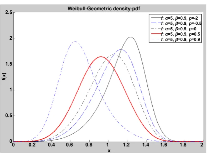
Figure 1. Shows Weibull-geometric density functions.

Figure 2. Displays Weibull-geometric cumulative functions.

respectively, with

β

=0.9 _and α=5 _{for the various rates of p. The EG} dis-tribution related to two-parameter with decreasing failure rate is introduced by Adamidis and Loukas [5]. When

α

=

1

and 0< <p 1_{, the exponential}

geome-tric (EG) distribution is obtained, and at

α

=

1

for any p<1 the EEG distri-bution is achieved. Therefore, the EEG distridistri-bution expands the EG distridistri-bution. The Weibull W

(

α β,

)

distribution is obtained when p goes to zero. Figure 1

plots the WG density for some values of the vector ϕ=

(

β α,

)

_when

2, 0.5,0,0.5,0.9

x→ ∞. The density functions of WG are shown. It is noted that the WG density is strictly decreasing when − ≤ <1 p 1 _and α≤1_{, and is multimodal when}

1 p 1

− ≤ < and α>1. The form 1 1 0

x _=β−u α _{is obtained when solution is}

ar-rived of the following nonlinear formulation:

(

)

1_eu _{1 1 1 1}

u p₊ − u_{− +} α _{= − +} α ₍₅₎

The WG density can be unimodal when p< −1_{. For instance, when} p< −1

and α=1_{, the EEG distribution is unimodal. The hazard and survival functions} of X are:

( )

(

)( )

₁

(

( ) 1

)

1 e t 1

h t _αβ p _βt α₋ p ₋β α−

= − − ₍₆₎

and

( )

(

( )

)

(

( ) 1

)

1 e t 1 e t 1 ,

S t ₋β α p ₋β α−

= − + − − ₍₇₎

3. Markov Chain Monte Carlo Algorithms

Markov chain Monte Carlo (MCMC) technique has spread widely for Bayesian calculation in compound statistical modeling. In general, it gives a beneficial ap-plication for real statistical modeling (Gilks et al. [20]; Gamerman, [21]).

Markov Chain is a randomly determined and stochastic process, having a random probability distribution or pattern that may be resolved statistically in that future cases are independent of previous cases specified the current case.

Monte Carlo chain is an emulation and simulation, therefore; it used to solve integrals to some extent rather than analyze performance, a procedure named integration of Monte Carlo. In this way, interested quantities of a distribution can be picked from emulated draws and charts from the distribution. Bayesian test needs integration over probably high-dimension of probability distributions to produce predictions or to yield inference and deduction about parameters of model. Basically, Monte Carlo integration is utilized with chains of Markov in MCMC techniques. The patterns of integration draw from the desired distribu-tion, and then form pattern rates to sacrificial expectations (see Geman [22]; Metropolis et al. [23]; and Hastings [24]).

3.1. MH Procedure

The Metropolis-Hastings (MH) procedure is employed by Metropolis et al.[23]. It is assumed that the main target here is to design samples from the distribution

(

|

)

( )

f τ x = ℘ τ , where is the normal fixed value which may be hard to calculate or found. MH procedure gives a method of sampling from f

(

τ|x

)

without the need to inform . Suppose that

(

_τ( )b _|τ( )a

)

_{is an optional}

transi-tion kernel, where the probability of jumping, or moving, from existing case

( )a

τ

to

_τ

( )b _{, known as the suggestion or proposal distribution. The MH}

Metropolis-Hastings Procedure

1) Select optional beginning value

_τ

( )0 _{for which f}

(

_τ( )0 _|x

)

_>0. 2) At time t sample candidate, points to or suggests that τ∗ _from

( )

(

_{τ τ}∗_| t−1

)

, the proposal distribution. 3) The approval probability is computed by:

( )

(

)

(

(

( )

)

)

(

(

( ) ( )

)

)

1 1

1 1

| |

, min 1, .

| |

t t

t t

f x

f x

τ τ τ

χ τ τ

τ τ τ

−

∗ ∗

− ∗

− ∗ −

 

 

=

 

 

(8)

4) Produce W W∼

( )

0,1 .

5) If _{W ≤χ τ}

(

( )t−1_,τ∗

)

_{, the suggestion is accepted and put}

_τ

( )t ₌

_τ

∗_{, else refuse}

the suggestion and put

_τ

( )t ₌

_τ

( )t−1 6) Repeat steps 2 - 5.

When the proposal distribution is symmetric, so

(

τ η|

)

=

(

η τ|

)

for all possible η and τ then, in particular, the result is

(

_τ( )t−1 _|τ∗

)

₌

(

_{τ τ}∗_| ( )t−1

)

_, so that the acceptance probability (5) is given by

( )

(

1

)

(

(

( )1

)

)

|

, min 1, .

|

t

t

f x

f x

τ χ τ τ

τ

∗

− ∗

−

 

 

=

 

 

(9)

3.2. GS Procedure

Gibbs’ sampler (GS) procedure is a straightforward branch of MCMC algo-rithms. This procedure was implemented by Geman [22]. The significance of Gibbs’ procedure for area of issues in Bayesian analysis is explained by Gelfand and Smith [25]. The complete conditional distribution forms the transition ker-nel, so Gibbs sampler procedure is a MCMC planner.

Gibbs sampling Procedure

1) Select optional beginning value ( )0

(

( )0 ( )0

)

1 , , d

τ = τ τ for which _℘

( )

_τ( )0 _>0. 2) By using conditional distribution

(

( )1 ( )1 ( )1

)

1| 2t , 3t , , dt

τ τ − τ − τ −

℘ , acquire τ1( )t . 3) By using conditional distribution

(

( ) ( )1 ( )1

)

2| 1t , 3t , , 1t

τ τ τ − τ −

℘ , acquire τ2( )t . 4) By using conditional distribution ℘

(

τ τ τ τd| 1( )t, 2( )t , 3( )t, ,τd( )t−1

)

, acquire τd( )t .

(5) Repeat steps 2 - 4.

4. MLE of WG Distribution

This section determines the maximum likelihood estimates (MLEs) of the WG distribution parameters. Let’s assume that Xi =Xi m nR; , ,i=1, 2, , m are the progressive first-failure censoring order statistics from a WG distribution, with censoring plane R. Using Equations (1)-(3), the function of likelihood is shown by:

(

)

(

)

(

)

(

) (

)

(

)

(

)

( ) 1 1 2 1

, , | 1 exp 1 log 1

1 exp i

m m

n

m m

i i i

i i

m R

i i

L p x p x x R

p x

α α

α

α β κα β α β

β = = − + =   = − × _ − − + _     × _ − − _

∑

∑

∏

(10)

where κ is given in (2). The logarithm of the function of likelihood may be obtained as follow:

(

)

(

)

(

)

(

) (

)

(

)

(

(

(

)

)

)

1 1

1

, , | log log log 1

1 log 1

2 log 1 exp .

m m

i i i

i i

m

i i

i

l p x m m n p

x x R

R p x

α

α

α β α α β

α β β = = = = + + − + − − + − + − −

∑

∑

∑

(11)

Compute the derivatives _∂∂_αl , _∂∂_βl and l

pα

∂

, then put each equation equal

to zero, the likelihood equations can be obtained in the following:

(

)

₍

_{)( )}

_{( )}

(

)( )

( )

(

( )

)

( )

(

)

1 1 1 , , |

log log 1 log

2 log exp

0, 1 exp

m m

i i i i

i i

m _{i i i i}

i _i

l p x _{m m}

x R x x

R x x x

p p x α α α α α β

β β β

α α

β β β

β = = = ∂ = + + − + ∂ + − − = − −

∑

∑

∑

(12)

(

)

₍

_{) ( )}

(

) ( )

(

( )

)

( )

(

)

1 1 1 1 , , | 1 2 exp 0 1 exp m

i i i

i

m _{i i i i}

i _i

l p x m _{R x x}

R x x x

p

p x

α

α α

α

α β _{α α}

β β β β β α β − = − = ∂ = − + ∂ + − − = − −

∑

∑

(13)

and

(

)

(

)

(

( )

)

( )

(

)

1 2 exp , , | 0,

1 _{1 exp}

m _{i i}

i _i

R x

l p x n

p p _{p x}

α α β α β β = + − ∂ − = + =

∂ −

∑

_{− −} (14)

The analytical solution of α βˆ, ˆ _and pˆ in Equations (12)-(14) is very diffi-cult. Hence, some numerical techniques like Newton’s method may be used.

From the function of log-likelihood in (11), the Fisher information matrix

(

, ,

)

(

)

(

(

)

1

(

)

)

0

ˆ ˆ

ˆ, ,pˆ N , , ,p I ˆ, ,pˆ ,

α β

_→

α β

−

α β

₍₁₅₎

where I0

(

α β, ,p

)

is observed as information matrix.

(

)

(

)

(

)

(

)

(

)

(

)

(

)

(

)

(

)

(

)

(

)

( )

( )

(

)

1

2 2 2

2

2 2 2

1

0 2

2 2 2

2

ˆ ˆ, ,ˆ

; , , ; , , ; , ,

; , , ; , , ; , ,

ˆ ˆ, ,ˆ

; , , ; , , ; , ,

ˆ

ˆ ˆ ˆ ˆ

var cov , cov , cov

p

l x p l x p l x p

p

l x p l x p l x p

I p

p

l x p l x p l x p

p p p

p

α β

α β α β α β

α β α

α

α β α β α β

α β

β α β β

α β α β α β

α β

α α β α

− −  ∂ ∂ ∂  − − −   ∂ ∂ ∂ ∂ ∂    _{∂ ∂ ∂}    = − − − ∂ ∂ ∂ ∂ ∂    _{∂ ∂ ∂}  _{− − −}   _{∂ ∂ ∂ ∂ ∂}    =

( )

( )

( )

(

)

( )

( )

ˆ_{,ˆ var} ˆ _{cov ,}ˆ _{ˆ .} ˆ

ˆ

ˆ ˆ ˆ

cov , cov , var

p

p p p

β α β β

α β               (16)

Confidence intervals can be calculated approximately for

α β

, _{and p to be}

bivariate normal distributed with the means

(

α β, ,p

)

and covariance matrix

(

)

1 0 ˆ, ,ˆ ˆ

I− α β p _{. Hence, the 100 1}

(

_−α

)

_{% confidence intervals approximately for} ,

α β

and p are

2 11 2 22 2 33

ˆ

ˆ z vα , z vα and p z vˆ α

α± β± ± ₍₁₇₎

respectively, where the values v11, v22 and v33 are on the major diagonal of the covariance matrix 1

(

)

0 ˆ, ,ˆ ˆ

I− α β p _and 2

zα is the percentage of the standard

normal distribution with right-tail probability α₂ .

5. Intervals of Bootstrap Confidence

The bootstrap technique is used for resampling in statistical inference cases. It is usually utilized to evaluate confidence regions and it can be applied to evaluate bias and variance of a calibrator or estimator assumption tests. Additional scan-ning of the parametric and nonparametric bootstrap technique is applied, see Davison and Hinkley [26], and Elhag et al. [27]. The parametric bootstrap tech-nique of the two confidence intervals is suggested. The algorithm for evaluating the confidence intervals of parameters uses both Efron and Tibshirani proce-dures [28], and bootstrap-t Hall procedure [20]. The Bootstrap sampling algo-rithm for estimating the confidence intervals of parameters is illustrated below.

Bootstrap Sampling Algorithm

1) Using the normal progressively Type-II samples, x=

(

x1<x2 <<xm

)

,

obtain α βˆ, ˆ, and pˆ, j=1, 2,3_.

2) Using the values of n and m (1<m n≤ ) with the same values of R,

(

i=1, 2, , m j

)

, =1, 2,3, generate random sample of sizes m from WG distri-bution, *

(

* * *

)

1 2 m

Continued

3) Use _x* _{as in step 1 to calculate the bootstrap sample estimates of α βˆ,} ˆ and pˆ indicated as _αˆ*_{, β}ˆ* _{and pˆ}*_.

4) By repeating the steps 2 and 3 N times, where N is the number of various bootstrap samples, put N = 1000.

5) Sort all values of _αˆ*_{, β}ˆ* _{and pˆ}* _{in an ascending order to get bootstrap} sample

(

* 1[ ]_, * 2[ ]_{, ,} *[ ]N

)

_{, 1, 2,3}

k k k k

ϕ ϕ ϕ = where

(

* * *

)

1 ˆ , 2 , 3 p .

ϕ ₌α ϕ∗ ₌β ϕ∗ ₌ ∗

Percentile bootstrap confidence interval: Assume that G y

( )

₌P

(

ϕˆ_j∗_≤y

)

is the cumulative distribution function of ϕˆ∗_{j. Determine ˆ} 1

( )

jboot G y

ϕ∗ ₌ − _for the given y. The bootstrap confidence interval approximately with 100 1

(

−γ

)

% of ϕˆ∗_{j may be obtained as follows:}

ˆ ,ˆ 1 .

2 2

jboot γ jboot γ

ϕ∗ ϕ∗

    ₋ 

   

 _{   }

  (18)

First, locate the sort statistics [ ]1 [ ]2 [ ]N_,

j j j

δ∗ _<δ∗ _<<δ∗ _wherever

[ ] [ ] [ ]

( )

ˆ ˆ

, 1, 2, , , 1, 2,3, ˆ

var

i

i j j

k

i j

i N j

ϕ ϕ δ

ϕ

∗ ∗

∗

−

= = = ₍₁₉₎

and ϕˆ1=α ϕˆ ˆ, 2=β ϕˆ,ˆ3= pˆ.

Consider that H y

( )

=P

(

δj∗< y

)

is the cumulative distribution function of

j

δ∗_{. If y is given, then}

( )

1

( )

ˆjboot t ˆj var ˆj H y .

ϕ ϕ ϕ −

− = + (20)

6. Bayes Estimation of the Model Parameters

In the consideration that each of the parameters

α β

, and p are unknown, it may be considered that the joint prior density is a product of gamma density of

α and

β

uniform prior of p, where

( )

_{( )}

1

(

)

(

)

1 exp , 0, , 0 ,

a a

b _{b a b}

a

π α ₌ α − ₋ α α_{> >}

Γ (21)

( )

_{( )}

1

(

)

(

)

2 exp , 0, , 0 ,

c c

d _{d c d}

c

π β ₌ β − ₋ β β _{> >}

Γ (22)

and

( )

3 p 1

π = (23) By multiplying π α1

( )

by π β2

( )

and π3

( )

p , we get the joint prior densi-ty of

α β

, and p computed by

(

_{, ,p}

)

_{( ) ( )}

b da c a1 c1_exp

(

(

_{b d}

)

)

_{, ,}

(

_{0 and 0 p 1 .}

)

a c

π α β ₌ α β− − ₋ α₊ β α β _{> ≤ ≤}

Γ Γ (24)

can be expressed as follows:

(

)

(

) (

)

(

) (

)

0 0 0

, , | , ,

, , | .

, , | , , d d d

L p x p

p x

L p x p p

α β

π α β

π α β

α β

π α β

α β

∗

∞ ∞ ∞

× =

×

∫ ∫ ∫

(25)

Hence, using squared error loss function (SEL) of any function ϕ α β

(

, ,p

)

_,

the Bayes estimate of

α β

, and p can be expressed as

(

)

(

(

)

)

(

) (

) (

)

(

) (

)

, , |

0 0 0

0 0 0

ˆ , , , ,

, , , , | , , d d d

, , | , , d d d

p x

p E p

p L p x p p

L p x p p

α β

ϕ α β ϕ α β

ϕ α β α β π α β α β α β π α β α β

∞ ∞ ∞ ∞ ∞ ∞ = × = ×

∫ ∫ ∫

∫ ∫ ∫

(26)

In general, the value of two integrals specified by (26) cannot be acquired in a cleared and closed format. In this situation, the MCMC procedure is used to create patterns from the posterior distributions and; therefore, is calculated the Bayes estimator of ϕ α β

(

, ,p

)

_{along with the function of SEL. A wide diversity}

of MCMC techniques is available and can be troublesome to select any of them. A significant type of MCMC technique is Gibbs samplers and widespread Me-tropolis within-Gibbs samplers.

The MCMC procedure has the advantage over the MLE procedure that we can permanently gain an appropriate estimation of intervals of the parameters by building the probability intervals and using the experimental posterior distribu-tion.

This, sometimes, is not obtainable in MLE. The samples of MCMC can be uti-lized to fully brief the uncertainty of posterior about the parameters

α β

, and

p, by using a kernel estimation of the posterior distribution.

The function of joint posterior density of

α β

, and p may be described as

(

)

(

)

(

)

(

(

)

)

(

)(

)

1 1

1

1 1

, , | 1 exp log

2 log 1 exp 1 .

m n

m a m c

i i

m m

i i i i

i i

p x p b d x

R p x R x

α

α α

π α β α β α β α

β β ∗ + − + − = = =  ∝ − − − +     − + _ − − _− + _   _

∑

∑

∑

(27)

The conditional posterior PDF’s of

α β

, and p are shown as

(

)

(

)

(

( )

)

(

)( )

1 1 1 1 1

| , , exp log log

2 log 1 exp 1 ,

m m a

i i

m m

i i i i

i i

p x m b x

R p x α R x α

π α β α α β

β β ∗ + − = = =    ∝ _{ } − + _       − + _ − − _− +  

∑

∑

∑

(28)

(

)

(

)

(

(

)

)

(

)(

)

1 2 1 1

| , , exp 2 log 1 exp

1 , m m c i i i m i i i

p x d R p x

R x

α α

α

π β α β β β

β ∗ + − = =  _{ } ∝ _− − + _ − − _     − +  

∑

∑

(29)

and

(

) (

)

(

)

(

( )

)

3

1

| , , 1 nexp m i 2 log 1 exp i .

i

p x p R p x α

π∗ α β β

=

 _{ }

∝ − − + _ − − _



∑

 (30)

under the Gibbs sampler algorithm is described as follows:

Gibbs/Metropolis-Hastings Sampler Algorithm 1) Initialize I=1_,

_α

( )0 ₌

_α

_{ˆ and β}( )0 _=βˆ_.

2) Based on Metropolis-Hastings, create

_α

( )I _{using (28) with the}

( )

(

1

)

1 ,

I

N α − σ _{proposal distribution, where}

1

σ _{is from}

variances-covariance matrix.

3) Based on Metropolis-Hastings, create _β( )I _{using (29) with the} ( )

(

1

)

2 ,

I

N β − σ _{proposal distribution, where}

2

σ _{is from}

variances-covariance matrix.

4) Based on Metropolis-Hastings, create _p( )I _{using (30) with the} ( )

(

1

)

3 ,

I

N p − σ _{proposal distribution, where}

3

σ _{is from}

variances-covariance matrix. 5) Calculate _α( )I ,_β( )I _{and p}( )I _.

6) Put I I= +1 .

7) Repeat steps (2 - 5) N times.

8) We get the point estimation by Bayes MCMC of ϕl (ϕ1=α ϕ, 2=β and

3 p

ϕ = _{) as}

(

)

( )

1

1

| N i,

l l

i M

E x

N M

ϕ

ϕ

= +

=

−

∑

(31)

where M is the number of iterations (burn-in period) before the stationary distribution is accomplished and posterior variance of ϕl becomes

(

)

(

( )

₍

₎

)

2

1

1

ˆ _| N i ˆ _{| ,}

l l l

i M

V x E x

N M

ϕ

ϕ

ϕ

= +

= −

−

∑

(32)

9) The quintiles of the pattern are picked as the endpoints of the interval to calculate the reliable intervals of ϕl. Sort ϕl(M+1),ϕl(M+2), ,ϕl( )N as

( )1, ( )2 , , ( )

l l l N M

ϕ ϕ ϕ ₋ . Hence, the symmetric credible interval with

(

)

100 1−γ % _is

( ) 1 ( )

2 2

,

l γ N M l γ N M

ϕ_{ } ϕ_{  }

− − −

    

    

 

 

 

  (33)

7. Illustrative Example and Simulation Studies

To explain the procedures evolved of estimation in this paper, gamma distribu-tion for given hybrid parameters (a=1.5,b=1_{) is used and produce sample of}

space 10, randomly (21), the average of the sample 10 1

1

10 i

i

α

α

=

≅

∑

_{, is computed}

and supposed as the real population rate of α =1.5_{. So that they are obtained to} verify E

( )

b

a

α = ≅α _{with the past parameters is nearly the average of gamma}

( )

2

π β _{based on the last}

β

=2_{, from gamma distribution (22). The previously}

parameters selected to verify E

( )

d c

β = ≅β _{, are nearly the average of gamma}

distribution. A progressive Type II samples are created by employing the proce-dures of Balakrishnan and Sandhu [19] from WG distribution with the available data: 0.0409, 0.0552, 0.0561, 0.0726, 0.0776, 0.0840, 0.0906, 0.1108, 0.1291, 0.1502, 0.1513, 0.1540, 0.1624, 0.1691, 0.1930, 0.2175, 0.2188, 0.2700, 0.2709, 0.2994, 0.3219, 0.3342, 0.4065, 0.4396, 0.5385, and under the parameters; (α =1.5_, p=0.6_,

β

=2_, m n= =50 _and

{

2,0, 2,0,1,0, 2,0,0,3,0,0, 2,0, 2,0,1,0,3,0,3,0, 2,0, 2

}

R= _).

[image:12.595.208.538.557.621.2]

The approximate bootstrap, Bayes estimates and MLEs are calculated of

α β

, , and p under these data utilizing MCMC algorithm outputs are explained in

Table 1 and Table 2. Table 2 yield the 95%, approximate confidence intervals of two bootstrap, approximate credible and MLE under the MCMC samples. Stu-dies of simulation have been executed employing Mathematica ver. 9.0 for ex-plaining the theoretic outcomes of estimates issue. The accomplishment of the performing estimators of the parameters has been supposed in valued of their mean square error (MSE) and average (AVG), where

( )

₍

₎

1 2 3

1

1

ˆ M ˆ , ,i , ,

k k

i

p M

ϕ

ϕ

ϕ α ϕ

β ϕ

=

=

∑

= = = ₍₃₄₎

and

( )

(

)

2

1

1 _ˆ

MSE M i .

k k

i

M =

ϕ

ϕ

=

∑

− (35) In studies of simulation, the researchers assume that the population parameter rates

(

α =0.5,β =1.5,p=0.1

)

, various sample values n, different effected sam-ple size m and different censored scheme R. For computing Bayes estimators, without loss of generality using non-informative priors, (a=0.0001, b=0.0001,

0.0001

c= _, d=0.0001_{). Under function of squared error loss, the researchers} calculate the Bayes estimations. The estimations of Bayes and 95% credible in-tervals using 11,000 sets of MCMC are also calculated. The mean Bayes estima-

Table 1. Show the parameters estimation of WG distribution.

Procedure α=1.5 β=2.0 p=0.6

(.)ML 1.6178 1.9614 0.4566

(.)Boot 1.8122 2.2451 0.7724

[image:12.595.207.541.653.732.2]

(.)MCMC 1.6299 1.9787 0.4727

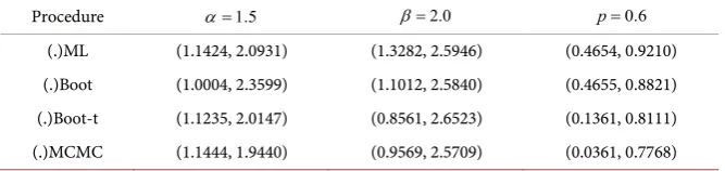
Table 2. Show the CIs using Bootstrap, Bootstrap-t and MLE according to 500 times.

Procedure α=1.5 β=2.0 p=0.6

(.)ML (1.1424, 2.0931) (1.3282, 2.5946) (0.4654, 0.9210)

(.)Boot (1.0004, 2.3599) (1.1012, 2.5840) (0.4655, 0.8821)

(.)Boot-t (1.1235, 2.0147) (0.8561, 2.6523) (0.1361, 0.8111)

tions, MSEs, coverage percentages, and average lengths of confidence interval based on 500 times are reported.

Comparatively, the MLEs with the 95% confidence intervals are calculated based on the observation of Fisher information matrix and two bootstrap confi-dences. Table 3 and Table 4 report the outputs based on MLEs and the Bayes estimations utilizing both the Gibbs sampling algorithm and MH algorithm:

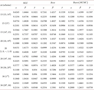
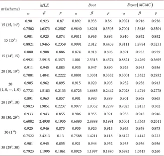
1) From Table 3 and Table 4, in parts of MSEs and credible intervals lengths, the estimators of Bayes depend on non-informative implement more effective than the MLEs and bootstrap.

2) From Table 3 and Table 4, comparing the models, the MSEs, average con-fidence interval lengths of the MLEs, and Bayes estimators for parameters are less significant for censored models

(

n m− ,0, ,0⋅⋅⋅

)

_.

3) The MSE and average confidence interval lengths nearly reduce the estima-tors in whole situations when the performance sample rate n m raises.

8. Conclusion

[image:13.595.208.537.418.735.2]

Several algorithms of estimation of WG distribution, based on the progressive Type II censored sampling plan, are discussed. The joint confidence intervals for the parameters are also studied. The approximate confidence regions, percentile bootstrap confidence intervals, as well as approximate joint confidence region

Table 3. Show the various estimators average values and the identical MSEs when

0.5, 1.5

α= β= _and p=0.1_.

m (scheme) MLE Boot Bayes MCMC

(

)

α β p α β p α β p

15 (15, 140₎ 0.6245 1.6664 0.1021 0.7241 1.4217 0.1539 0.5241 1.4399 0.1597

0.1234 0.4736 0.0664 0.2235 0.4840 0.1021 0.1200 0.1914 0.1056

15 (151₎ 0.6754 1.6828 0.1016 0.6788 1.4027 0.1482 0.5751 1.4194 0.1533

0.2101 0.5398 0.0614 0.2479 0.5438 0.0906 0.1101 0.4530 0.0936

15 (140_{, 15)} 0.5364 1.7667 0.1001 0.5388 1.3614 0.1554 0.5064 1.3977 0.1621

0.2351 0.7337 0.0707 0.3331 0.8748 0.1069 0.1111 0.5925 0.1105

20 (10, 190₎ 0.6200 1.6165 0.1023 0.7070 1.4327 0.1432 0.5205 1.4424 0.1471

0.1088 0.3890 0.0623 0.1282 0.3347 0.0874 0.0988 0.3389 0.0596 20

(1, 0, ···, 1, 0)

0.6151 1.6173 0.1024 0.6999 1.4234 0.1404 0.5151 1.4322 0.1439 0.1901 0.4028 0.057 0.2220 0.4500 0.0793 0.1102 0.3543 0.0511

20 (190_{, 10)} 0.6164 1.6782 0.0968 0.7162 1.4204 0.1400 0.5146 1.4375 0.1443

0.2225 0.5091 0.0577 0.2335 0.6194 0.0813 0.1325 0.4272 0.0537

30 (30, 290₎ 0.5777 1.7881 0.0974 0.7357 1.4828 0.1297 0.5577 1.4934 0.1320

0.1100 0.7534 0.054 0.2102 0.7296 0.0707 0.0985 0.6377 0.0518

30 (130₎ 0.6360 1.9606 0.094 0.5399 1.5464 0.1233 0.6355 1.5575 0.1254

0.1840 1.0418 0.0447 0.1990 0.9999 0.0570 0.1000 0.8539 0.0480

30 (290_{, 30)} 0.6321 2.1049 0.0950 0.6355 1.4381 0.1320 0.6333 1.4661 0.1351

[image:14.595.207.538.101.415.2]

Table 4. Show the coverage percentages and average confidence interval, when

0.5, 1.5

α= β= and p=0.1.

m (scheme) MLE Boot Bayes MCMC

(

)

α β p α β p α β p

15 (15, 140₎ 0.90 0.923 0.87 0.892 0.933 0.86 0.9021 0.916 0.936

0.7502 1.6373 0.2507 0.9840 1.8201 0.3503 0.7001 1.5616 0.3504

15 (151₎ 0.901 0.923 0.874 0.9011 0.963 0.894 0.910 0.952 0.952

0.8821 1.9465 0.2358 0.9991 2.012 0.4458 0.8111 1.8784 0.3231

15 (140_{, 15)} 0.880 0.908 0.886 0.874 0.918 0.896 0.891 0.933 0.939

0.9921 2.5915 0.3571 1.001 2.5313 0.4574 0.8821 2.4269 0.3695

20 (10, 190₎ 0.911 0.945 0.883 0.933 0.947 0.890 0.924 0.943 0.936

0.7001 1.4041 0.2222 0.8801 1.3331 0.3332 0.3001 1.3522 0.2932 20

(1, 0, ···, 1, 0)

0.905 0.962 0.895 0.915 0.920 0.905 0.932 0.958 0.943

0.7721 1.5183 0.2133 0.8723 1.6683 0.2442 0.7028 1.4749 0.2778

20 (190_{, 10)} 0.891 0.963 0.857 0.901 0.980 0.889 0.901 0.968 0.965

0.9823 1.9051 0.2237 0.9977 1.9352 0.2299 0.7023 1.8133 0.302

30 (30, 290₎ 0.933 0.943 0.855 0.906 0.955 0.921 0.935 0.945 0.946

0.6002 2.4938 0.1935 0.6880 2.8888 0.1991 0.5001 1.4563 0.2011

30 (130₎ 0.925 0.946 0.873 0.933 0.920 0.913 0.965 0.959 0.975

0.7522 3.4213 0.13 0.7588 1.4211 0.118 0.6122 1.4142 0.223

30 (290_{, 30)} 0.901 0.945 0.855 0.921 0.944 0.952 0.933 0.956 0.956

0.7923 1.1995 0.1061 0.8925 1.1997 0.1880 0.6982 1.0515 0.260

for the parameters are expanded and developed. Some numerical examples with actual data set and simulated data are used to compare the proposed joint confi-dence regions. The parts of MSEs and credible intervals lengths, the estimators of Bayes depend on non-informative implement more effective than the MLEs and bootstrap. Comparing the models, the MSEs, average confidence interval lengths of the MLEs, and Bayes estimators for parameters are less significant for censored models.

References

[1] Al-jibory, W.K.S. and EI-Zaart, A. (2013) Edge Detection for Diagnosis Early Alz-heimer’s Disease by Using Weibull Distribution. 25th International Conference on Microelectronics (ICM), Beirut, 15-18 December 2013.

[2] Scholte, H.S. and Ghebreab, S. (2009) Lourens Waldorp. In: Arnold, W.M.S. and Victor, A.F.L., Eds., Brain Responses Strongly Correlate with Weibull Image Statis-tics When Processing Natural Images, Vol. 9, 29. https://doi.org/10.1167/9.4.29

[3] El-Sayed, M.A., Abd-Elmougod, G.A. and Abdel-Khalek, S. (2013) Bayesian and Non-Bayesian Estimation of Topp-Leone Distribution Based Lower Record Values. Far East Journal of Theoretical Statistics, 45, 133-145.

[4] Afify, A.Z., Nofal, Z.M. and Butt, N.S. (2014) Transmuted Complementary Weibull Geometric Distribution. Pakistan Journal of Statistics and Operation Research, 10, No. 4.

Rate. Statistics and Probability Letters, 39, 35-42.

[6] Kus, C. (2007) A New Lifetime Distribution. Computational Statistics & Data Anal-ysis, 51, 4497-4509.

[7] Chahkandi, M. and Ganjali, M. (2009) On Some Lifetime Distributions with De-creasing Failure Rate. Computational Statistics and Data Analysis, 53, 4433-4440. [8] Tahmasbi, R. and Rezaei, S. (2008) A Two-Parameter Lifetime Distribution with

Decreasing Failure Rate. Computational Statistics and Data Analysis, 52, 3889-3901. [9] Barreto-Souza, W. (2011) The Weibull-Geometric Distribution. Journal of

Statistic-al Computation and Simulation, 81, 645-657.

https://doi.org/10.1080/00949650903436554

[10] Morais, A.L. and Barreto-Souza, W. (2011) A Compound Class of Weibull and Power Series Distributions. Computational Statistics and Data Analysis, 55, 1410- 1425.

[11] Barreto-Souza, W. and Cribari-Neto, F. (2009) A Generalization of the Exponen-tial-Poisson Distribution. Statistics and Probability Letters, 79, 2493-2500.

[12] Louzada, F., Roman, M. and Cancho, V.G. (2011) The Complementary Exponential Geometric Distribution: Model, Properties, and Comparison with Its Counterpart. Computational Statistics and Data Analysis, 55, 2516-2524.

[13] Cancho, V.G., Louzada-Neto, F. and Barriga, G.D.C. (2011) The Poisson-Expo- nential Lifetime Distribution. Computational Statistics and Data Analysis, 55, 677- 686.

[14] Hamedani, G.G. and Ahsanullah, M. (2011) Characterizations of Weibull Geome-tric Distribution. Journal of Statistical Theory and Applications, 10, 581-590. [15] Wang, M. and Elbatal, I. (2015) The Modified Weibull Geometric Distribution.

METRON, 73, 303-315.

[16] El-Din, M.M., Riad, F.H. and El-Sayed, M.A. (2014) Confidence Intervals for Para-meters of IWD Based on MLE and Bootstrap. Journal of Statistics Applications & Probability, 3, 1-7.

[17] El-Din, M.M., Riad, F.H. and El-Sayed, M.A. (2014) Statistical Inference and Pre-diction for the Inverse Weibull Distribution Based on Record Data. International Journal of Advanced Statistics and Probability, 3, 171-177.

[18] Elhag, A., Ibrahim, O.I.O. and, El-Sayed, M.A. (2014) Some Features of Joint Con-fidence Regions for the Parameters of the Inverse Weibull Distribution. Mathemat-ical Theory and Modeling Journal, 4, 118-124.

[19] Balakrishnan, N. and Sandhu, R.A. (1995) A Simple Simulation Algorithm for Ge-nerating Progressively Type-II Censored Samples. The American Statistician, 49, 229-230.

[20] Gilks, W.R., Richardson, S. and Spiegelhalter, D.J. (1996) Markov Chain Monte Carlo in Practices. Chapman and Hall, London.

[21] Gamerman, D. (1997) Markov Chain Monte Carlo: Stochastic Simulation for Baye-sian Inference. Chapman and Hall, London.

[22] Geman, S. and Geman, D. (1984) Stochastic Relaxation, Gibbs Distributions, and the Bayesian Restoration of Images. IEEE Transactions on Pattern Analysis and Mathematical Intelligence, 6, 721-741.

https://doi.org/10.1109/TPAMI.1984.4767596

[24] Hastings, W.K. (1970) Monte Carlo Sampling Methods Using Markov Chains and Their Applications. Biometrika, 57, 97-109. https://doi.org/10.1093/biomet/57.1.97

[25] Gelfand, A.E. and Smith, A.F.M. (1990) Sampling Based Approach to Calculating Marginal Densities. Journal of the American Statistical Association, 85, 398-409.

https://doi.org/10.1080/01621459.1990.10476213

[26] Davison, A.C. and Hinkley, D.V. (1997) Bootstrap Methods and Their Applications. 2nd Edition, Cambridge University Press, Cambridge.

https://doi.org/10.1017/CBO9780511802843

[27] Elhag, A.A., Ibrahim, O.I., El-Sayed, M.A. and Abd-Elmougod, G.A. (2015) Estima-tions of Weibull-Geometric Distribution under Progressive Type II Censoring Samples. Open Journal of Statistics, 5, 721-729.

https://doi.org/10.4236/ojs.2015.57072

[28] Efron, B. and Tibshirani, R.J. (1993) An Introduction to the Bootstrap. Chapman and Hall, New York.https://doi.org/10.1007/978-1-4899-4541-9

Submit or recommend next manuscript to SCIRP and we will provide best service for you:

Accepting pre-submission inquiries through Email, Facebook, LinkedIn, Twitter, etc. A wide selection of journals (inclusive of 9 subjects, more than 200 journals)

Providing 24-hour high-quality service User-friendly online submission system Fair and swift peer-review system

Efficient typesetting and proofreading procedure

Display of the result of downloads and visits, as well as the number of cited articles Maximum dissemination of your research work