Asymptomatic Distribution of Goodness of Fit Tests in Logistic Regression Model

http://www.scirp.org/journal/ojs ISSN Online: 2161-7198

ISSN Print: 2161-718X

Asymptomatic Distribution of Goodness-of-Fit

Tests in Logistic Regression Model

Nuri H. Salem Badi

Mathematics Department, Faculty of Art and science-Alabyar University of Benghazi, Benghazi, Libya

Abstract

The logistic regression model has been become commonly used to study the association between a binary response variable; it is widespread application rests on its easy application and interpretation. The subject of assessment of goodness-of-fit in logistic regression model has attracted the attention of many scientists and researchers. Goodness-of-fit tests are methods to deter-mine the suitability of the fitted model. Many of methods proposed and dis-cussed for assessing goodness-of fit in logistic regression model, however, the asymptotic distribution of goodness-of-fit statistics are less examine, it is need more investigated. This work, will focus on assessing the behavior of asymp-totic distribution of goodness-of-fit tests, also make comparison between global goodness-of-fit tests, and evaluate it by simulation.

Keywords

Logistic Regression Model, Goodness-of-Fit Tests

1. Introduction

The goal of a logistic regression analysis is to find the best fitting model to de-scribe the relationship between an outcome and covariates where the outcome is dichotomous, [1] considered the logistic regression model is a member of the class of the generalized linear models. Many assumptions and more details con-sidered about the behavior of logistic model see [2][3], also for more application see [4][5] [6][7]. The goodness-of-fit is very important to decide if the more succinct model is adequate. After fitting the logistic regression model, the next step is to examine the proposed model how well fits the observation data and to know how effective the model is; this is called as its goodness-of-fit. Good-ness-of-fit tests for the logistic regression can be split into three types: 1) Those based an examination of residuals; 2) Those based a test which groups the

ob-How to cite this paper: Badi, N.H.S. (2017) Asymptomatic Distribution of Goodness-of- Fit Tests in Logistic Regression Model. Open Journal of Statistics, 7, 434-445.

https://doi.org/10.4236/ojs.2017.73031

Received: April 17, 2017 Accepted: June 9, 2017 Published: June 12, 2017

Copyright © 2017 by author and Scientific Research Publishing Inc. This work is licensed under the Creative Commons Attribution International License (CC BY 4.0).

servation; 3) Those which do not group observation. Methods in 1) are more general and subjective assessments of a model and are not considered in this work. This is not to undervalue then they are often the most valuable approach to model assessment. The observed values for Bernoulli regression are just 0 s and 1 s and this makes graphical approaches less easy to handle. The focus of this work is the test statistics. In next section, tests using grouping are consi-dered, with those that do not need to group the data being discussed in section 3. Investigate the behavior of the asymptotic distribution of goodness-of-fit tests is considered in section 4 with comparisons between some goodness-of-fit tests, evaluated by simulation data with two different sample sizes. The simulation in this work was designed according to simulation that made by [8], which made comparisons between some goodness-of-fit tests in logistic regression models with sparse data. The results of his simulation showed that some goodness-of-fit tests have reasonable power compared with other tests. However, Kuss did not give information about the asymptotic distribution of these statistics. This paper supposes to show the behavior of the asymptotic distribution of goodness-of-fit tests for logistic regression model. Finally, conclusion and further discussion made in the last section.

2. Goodness-of-Fit Tests with Grouping

[9] proposed and developed approaches involving grouping based on the values of the estimated probabilities obtained from the fitted logistic model. Two grouping methods were proposed. The first approach is based on grouping the data according to percentiles of the estimated probabilities, and the second ap-proach is based on grouping the data according to fixed cutoff values of the es-timated probabilities. Tests with grouping based on eses-timated probabilities were proposed and developed by [9] [10] [11]. [12] developed a score test statistic which essentially compares two fitted model.

Hosmer and Lemeshow Test _Cˆ _{The calculation of this test dependent upon}

grouping of estimated probabilities πˆ

( )

x_i which use g groups. The first group

contains the n1=n g observations which have the smallest estimated

probabil-ities, the second group contains n2=n g values have the next smallest

esti-mated probabilities and the last group contains the n_g =n g observation with

the largest πˆ

( )

x_i : here n is the size of the sample and g the total number of

groups. Before defining a formulae to calculate _Cˆ _{we will consider some}

no-tions. The statistic test _Cˆ _{is obtained by calculating Pearson chi-square statistic}

from the 2×g table with two rows and g columns of observed and expected

frequencies. In the row with y = 1 summing of the all estimated probabilities in a group give the estimated expected value. In the row with y = 0 estimated ex-pected value is obtained by summing one minus the estimated probabilities over all subjects in the group. We can denotes the observed number of subjects have had the event present

(

y=1

)

and absent

(

y=0

)

respectively in each group

(

)

1 0

1 1

, 1

= =

=

∑

ns =

∑

ns −

s i s i

i i

O y O y

where ns is the number of the observation in group g. The expected number of subjects of present and absent respectively is denoted by:

(

)

1 0

1 1

ˆ, 1 ˆ

π π

= =

=

∑

ns =

∑

ns −

s i s i

i i

E E

Then _Cˆ _{is simply obtained by calculation the Pearson} χ2 _{statistic for the}

observed and expected frequencies from the 2×g table as:

(

)

2

1

1 0

ˆ g js js

s j js

O E

C

E = =

−

=

∑∑

from which it following

(

) (

2

)

2

0 0 1 1

1 0 1

ˆ

=

 _{− −} 

 

= +

 

 

∑

g s s s s

s s s

O E O E

C

E E

and finally we get

(

)

(

)

2

1

ˆ _,

1

π

π

π

= − =

−

∑

g s s s s s s s

O n C

n

where, ns is the total number of values in sth group, Os is the number of res-ponses for the number of covariates in the sth _{group, defining as}

1 = =

∑

ns

s i

i

O y

where, Os=O1s+O0s, and πs is the average of the estimated probabilities which are defined as:

1 ˆ

. s

n i i s

i s

m n

π π

=

=

∑

Here, the number of observations within covariate pattern i is denoted by mi. Use of an extensive set of simulations proved that when mi =1, where mi is the individual binomial denominator and the fitted logistic model is the correct model, then the distribution of _Cˆ _{is approximated by the} χ2 distribution

with

(

g−2

)

degrees of freedom [9].

Hosmer and Lemeshow Test _Hˆ

The second grouping strategy was proposed from Hosmer and Lemeshow denoted by _Hˆ _{, this method depends upon grouping the estimated probabilities}

in groups based on fixed cutpoint, so each group contains all subjects with fitted probability located in specific intervals. For example, the cutpoint of the first group is 0.0≤πˆ

( )

xi <0.1, then this group contains all subjects with estimated

probabilities located in this interval; the second group contains all subjects with estimated probabilities located between cutpoint 0.1≤πˆ

( )

xi <0.2 and the last

group has interval 0.9≤πˆ

( )

xi <1.0.

The calculation of _Hˆ _{uses exactly the same formulae used to calculate C}ˆ_:

groups. The distribution of _Hˆ _{is approximated by the} χ2 _{distribution with}

(

g−2

)

degrees of freedom.

Although Hosmer and Lemeshow tests are good, it requires grouping, and choice of g is

• _{g is arbitrary but almost everywhere in the literature and in software a value}

of 10, or very similar is chosen.

• _{Smaller values of g might be chosen for smaller n.}

• _{Sparse data causes a problem for H and lead to uneven group widths for C.}

3. Goodness-of-Fit Tests without Grouping

Deviance and Pearson Chi-Square Tests

Two of the most commonly used goodness-of-fit measures, are the Pearson’s chi-squared χ2 and the deviance D goodness-of-fit test statistics but the

beha-viour of these tests are unstable with bernoulli data; see [13]. The general idea of the deviance is make comparison between two models the first model is full model with p parameters and the second model is a model with q parameters, where

(

q< p

)

. The deviance can write as

(

)

ˆ

2 log 2 ,

ˆ

 

= − _ _= − −

   

s

s r r

L D

L

where ˆ

r

L , Lˆs are the likelihoods for the full and small model and r, s denoted to the log-likelihood: Asymptotically this is χ2 _{in −}

p q df. The

re-sidual deviance is the case when the large model is saturated and has n parame-ters. In case of the logistic regression model [13] introduced specific form when

1

=

i

m ; the residual deviance can then be found as

(

) (

)

{

}

1

ˆ ˆ ˆ ˆ

2 π logπ 1 π log 1 π ,

=

= −

∑

n i i+ − i − i

i

D

In this case the deviance is invalid as a goodness-of-fit test, because it is a function of πˆi, which does not compare the observed values with fitted values.

Also, [13] discussed that Pearson chi-square goodness of fit statistic when

1

=

i

m ; can be written:

(

)

(

)

2 2

1

ˆ

ˆ 1 ˆ

π

π

π

= −

= =

−

∑

n i i

y

X n

which is equal to the sample size: this is not a useful goodness-of-fit test.

Residual Sum of Squares Test

[14] proposed a method, which used the unweighted residual sum of squares a goodness-of-fit test to assess the model adequacy. The idea of this approach is to keep all the individual values of mi but to give less weight in cases of mi are small.

The unweighted residual sum of squares statistic considers only the numerator of the Pearson chi-squares statistic, which is the summation again over the indi-vidual observations, the statistic can be written:

(

)

2

1

ˆ .

π = =

∑

n _i− _i

i

Of course, the relative weighting for varying mi is not relevant for our case

where mi = 1. [11] discussed how to compute the moments and asymptotic

distri-bution of the RSS statistic. They give useful expressions for the mean and variance which are easier to compute than the expressions given by [14]. The proposed asymptotic mean and variance of RSS are respectively, E RSS_ −S W

( )

_≅0

and var _{ −}

( )

_≅ T

(

₋

)

RSS S W  d I M Wd, where M =WX X WX

(

T

)

−1XT,

(

)

diag

π

1

π



= _ i − i _

W , S W

( )

=

∑

in₌₁_diag

(

πi

(

1−πi

)

)

_ and d is vector with

elements di= −

(

1 2πi

)

. Used the standardized statistic to assess significance by referring the following to the standard normal

( )

( )

. var

−

 

 

−

 

 

RSS S W

RSS S W

2

R Test

Several 2

R type statistics have been used for goodness-of-fit in logistic

re-gression, such as that proposed by [15].

2 2

0

ˆ 1

ˆ

 

= −  _{ }

 

n c g

L R

L

where, ˆ

c

L represents the log-likelihood evaluated at the ML estimation

para-meters and Lˆ0 represents the log-likelihood of the model containing only an

intercept. Another version due to [16] is

( )

2 2

2

max

= g

g

g

R R

R

where,

( )

( )

2 2

0 ˆ max Rg = −1 L n.

Information Matrix tests: IMT and IMTDIAG

The Information Matrix test (IMT) is a test for general mis-specification, proposed by [17]. The two well-known expressions for the information matrix coincide only if the correct model has been specified and the IMT takes advan-tage of this fact. The IMT avoids the grouping necessary for tests like the Hos-mer-Lemeshow test. Many researchers, [18][19][20][21] pointed out the beha-viour of the asymptotic distribution of IMT statistic and dispersion matrix. [22]

discussed the information matrix test and showed that it is useful with binary data models. [8] claimed that, the IMT has reasonable power compared with other tests, without information about the behaviour of the asymptomatic dis-tribution of IMT. The idea of the information matrix test is to compare

2

T

E

θ θ

 −∂ 

_{∂ ∂} 

 

 _and

T θ θ ∂ ∂

 

_{∂ ∂} 

 

 

E , as these differ when the model is mis-specified

but not when the model is correct.

Let, consider binary regression, where the outcome for individual i, i = 1, ···, n

is a random variable Yi∈

{ }

0,1 . Also

(

)

( )

T

Pr Y xi| i =

π

i = f xi

β

where xi is a

1

×

p dimensional vector of covariates and β is a p-dimensional vector of

pa-rameters. It will be convenient to write ₌ Tβ

i i

We have

( )

( )

(

) (

)

1 1

log 1 log 1

β β π π

= =

=

∑

=

∑

+ − −

 n i n i i i i

i i

Y Y

The p-dimensional likelihood equations ∂ ∂ = β 0 can be written:

(

)

(

)

1 0 1 π π

β = π π

 − ∂

∂ _{= =}

 

∂

∑

_ − _∂

n

i i i

i

i i i i

Y

x

a (1)

We can also derive the p×p matrix ∂2 ∂ ∂β βT as:

(

)

(

)

(

(

)

)

2 2

2

1 1 T

2 ₂ 2

1 1 1

π π π π

π π _{π π}

=  _{− ∂ − ∂ }   − _{ }  − ∂ ∂  −     

∑

n i i i i

i i

i i i i i i i

Y Y

x x a

a (2)

The idea behind the information matrix test is that if the model is correctly specified then the quantity:

2

T T

1 β β βˆ β β βˆ

= _{∂ ∂ ∂}    = + ∂ ∂ ∂ ∂   

∑

n i i i i

IM

has zero mean. By comparing (1) and (2) we can compute this quantity, for a general value of β_{, as the sum of:}

(

)

(

)

2 2

T

T T 2

1

π π

β β β β π π

−

∂ ∂ ∂ ∂

+ =

∂ ∂ ∂ ∂ − ∂

i i

i i i i

i i

i i i

Y

x x

a (3)

We can test the null hypothesis that IM has zero mean by computing the va-riance of IM and then constructing a standard χ2 _{statistic. The first step is to}

compute the variance of −12

∑

i

n d where we write di for essentially the right hand side of (3):

(

)

(

)

2 2 1 π π π π − ∂ − ∂

i i i

i

i i i

Y

z a

where we have changed the p×p symmetric matrix into a vector z_i in order

to be able to use standard methods. As T

i i

x x is symmetric we do not wish to

duplicate entries, so zi is the

(

)

1

1

2p p+ -dimensional vector:

( ) ( ) ( )

(

)

T

11, 21, , 1 , 22, 32, , 2 , , −1 , −1, , −1,

     

=           

i p p p p p p pp

z x x x x x x x x x

where xst is the

( )

, th

s t element of x xi iT. If we write:

(

)

(

)

(

)(

)

1 1 2

2 2 2 1 1 2 1 1 1 2 π π π π π π − − = − = − ∂ = = − ∂ = − −

∑

∑

∑

n

i i i

i i

i i i i

n

i i i

i

Y

A n d n z

a

n Y z

then because the different terms are independent we obtain:

( )

₍

₎

2 2 T

2 1 1 1 var . 1 π π π = ∂ 

Ψ = = ₋ _∂ 

 

∑

n

i i i

i i i i

A z z

which is a q q× dimensional matrix where 1

(

1

)

2

= +

q p p .

We should also note that if B is defined as essentially the log-likelihood, i.e.

(

)

(

)

(

)

1 1

2 2

1 1 1

π

π

_π

π

π

− − = = − ∂ = = − − ∂

∑

n i i i

∑

n

i i i i

i i i i i

Y

B n x n Y x

a

then the variance of B is the p×p matrix Ω:

(

)

2 T 1 1 1 1 π π π = ∂ 

Ω = _{ }

− _∂ _

∑

n

i i i

i i i i

x x

n a

Before compute the covariance of A and B, we get, using

(

) (

2

) (

)(

)

1 1 2

π π

π

π

π

− − = − −

i i i i i i i

y y

Now,

(

)

( )

( ) ( )

cov A B, =E AB −E A E B

For independently and identically random variables and under the H0 the

second term of the cov

(

A B,

)

is zero, and covariance of A and B in this case is

the q×p matrix, and so

(

)

₍

₎

2 T

2 1 1 1 cov , 1

π

π

π

π

=   ∂  ∂ ∆ = = _{  } − _∂ _ ∂ _

∑

n i i

i i

i i i i i

A B z x

n a a

Central limit arguments suggest that asymptotically

(

T T

)

,

A B is a q+p

dimensional normal variable. However, the IM-test requires A to be evaluated at

ˆ

β_{, A}ˆ_{, say, and at this value we know that B = 0. Consequently the variance of} ˆ

A is the variance of A conditional on B = 0 which is Ψ − ∆Ω ∆−1 T.

Assuming a logistic regression we have ∂πi ∂ =ai πi

(

1−πi

)

and

2 2

i ai

π

∂ ∂

(

1

)(

1 2

)

i i i

π π π

= − − so we can evaluate the dispersion matrices at the MLEs as:

(

)

T

1

1

ˆ _{πˆ 1 πˆ}

=

Ω =

∑

n _i − _{i i i}

i

x x n

(

)(

)

2 _T

1

1

ˆ _{πˆ 1 πˆ 1 2πˆ}

=

Ψ =

∑

n _i − _i − _{i i i}

i

z z n

(

)(

)

T

1

1

ˆ _{πˆ 1 πˆ 1 2πˆ}

=

∆ =

∑

n _i − _i − _{i i i}

i

z x n

If we write _{ˆ= Ψ − ∆Ω ∆ˆ ˆ ˆ}−1_ˆT

V then one version of the IM test is found by

re-ferring _ˆT_ˆ−1_ˆ

A V A to a χ2 variable with degrees of freedom equal to the rank of

ˆ

V.

The idea of the IMDIAG test and IM test are the same, the only difference is that

for the former the elements of zi are just the diagonal elements of

T

i i

x x , so zi is the p dimensional vector:

(

)

T 2 2 2

1, 2, , .

= 

i i i ip

z x x x

To explain the difference in size of vector zi in the two cases of IM test and

IMDIAG test, let us consider a simple example. Suppose we have a symmetric

ma-trix with elements T

i i

11 12 13 21 22 23 31 32 33

,

 

 

 

 

 

x x x

x x x

x x x

where, x_rs =x x_{ri si}. Then in the case of the IM test, the dimension of vector ziT is 1 6× and elements are:

[

]

T

11, 12, 13, 22, 23, 33 , =

i

z x x x x x x

whereas in the case of IMDIAG test, zi is the 1 3× dimensional vector:

[

]

T

11, 22, 33 . =

i

z x x x

4. Simulation Study

Our work, focus on behaviour of goodness of fit tests under alternative hypo-theses in case of missing covariate model and in case of the wrong model, be-cause these cases we could not reproduce Kuss’s work in. We will focus on four goodness-of-fit tests

(

Cˆ ,_g RSS IM IM, , _DIAG

)

. Therefore, we examine in more

depth the behaviour of the tests and determine more information about asymp-totic MLE distribution in case of the wrong model

(

2

)

expit 0.405 ,

π

i= xi

or in the case of the missing covariate,

(

)

expit 0.405 0.223 ,

π =i xi + ui

where X U, ~U

(

−6, 6

)

, X and U independent.

Simulation study designed as Kuss’s work:

• _{The sample sizes are n = 100 and n = 500.}

• _{Applied only on extreme sparseness when} mi =1. • _{number of simulation is 1000.}

• _{distribution of the predictor variables X, U is} U

(

−6, 6

)

, X and U

indepen-dent chosen to confirm with Kuss’s work.

• _{Use four of goodness-of-fit tests from the simulation study under three}

dif-ferent alternative hypotheses: (a) True covariate.

(b) Missing covariate.

(c) Wrong functional form of the covariate.

• _{Fitted model in all cases is a standard logistic model with an intercept and}

one covariate.

• _{All the tests on the null hypothesis under} α =0.05.

Results and Discussion of Tests under Correct Model

In Table 2, reported some results, the mean, variance and the empirical power of four goodness-of-fit tests from simulation study under correct model, namely

(

)

expit 0.693 .

π =i xi

Statistics used in the simulation as goodness-of fit tests are: Hosmer- Lemeshow

( )

ˆ

g

(

IMDIAG

)

and residual sum of squares (RSS). The asymptotic distribution of

statistics is 2

df

χ

distribution, where the mean and variance equal df and 2df

respectively. In case of

( )

ˆ

g

C statistic we chosen the number of group is g = 10

so, degree of freedom is df = −g 2. The results shown in Table 1, the mean

and variance of all statistics appeared close to df and 2df. Moreover, the simula-tion study appeared reasonable results when fit the model with sample size n = 500. However, there is slightly large variance of

( )

ˆ

g

C in case of sample size n =

100. Overall, the empirical power and type I error looks good.

In the second case, the results reported the mean, variance and the power to detect a mis-specified model for same goodness-of-fit tests under missing cova-riate model, when the model is:

( )

(

)

logit π =i expit 0.405xi+0.223ui ,

[image:9.595.207.541.481.584.2]

and fit standard logistic regression model with xi.

Table 2, showed results from simulation study under alternative hypotheses missing covariate model. The mean and variance of all statistics close to df and 2df, but we have slightly smaller variance in case of ˆ

g

C . However, we have low

power when used IM statistics in case of sample size n = 500, IMDIAG statistic and RSS in case of sample size n = 100 and ˆ

g

C statistic in both cases of sample size.

The final case we will show the results of power to detect a mis-specified model for four goodness-of-fit tests under the wrong functional form of the co-variate model

( )

(

2

)

logit

π

_i =expit 0.405x_i

and fit the model as previous cases.

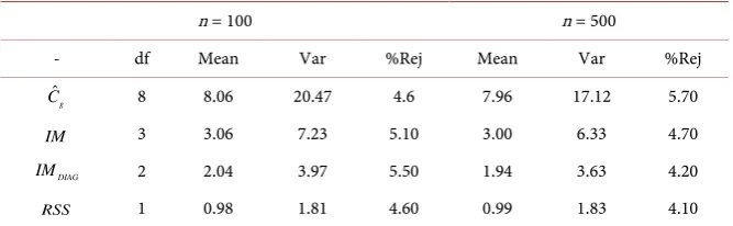
Table 1. Results of N = 1000 simulation with sample size n = 100 and n = 500 under correct model.

n = 100 n = 500

- df Mean Var %Rej Mean Var %Rej

ˆ

g

C 8 8.06 20.47 4.6 7.96 17.12 5.70

IM 3 3.06 7.23 5.10 3.00 6.33 4.70

DIAG

IM 2 2.04 3.97 5.50 1.94 3.63 4.20

[image:9.595.205.542.630.733.2]

RSS 1 0.98 1.81 4.60 0.99 1.83 4.10

Table 2. Results of N = 1000 simulation with sample size n = 100 and n = 500 under missing covariate model.

n = 100 n = 500

- df Mean Var %Rej Mean Var %Rej

ˆ

g

C 8 7.44 11.13 1.50 7.35 12.62 3.20

IM 3 3.01 6.05 5.50 2.38 4.15 1.90

DIAG

IM 2 1.82 3.06 3.3 2.05 3.46 4.80

In Table 3, reported results for goodness-of-fit tests from simulation study under wrong model. The mean and variance of all statistics appeared very larger in two cases of sample size comparing with degree of freedom of statistics. How- ever, high power in all goodness-of-fit tests in both sample size were found, that is meaning this tests have rejected all the null hypothesis. On the other hand, Kuss’s results appeared low power in case of sample size n = 100 compared with our results.

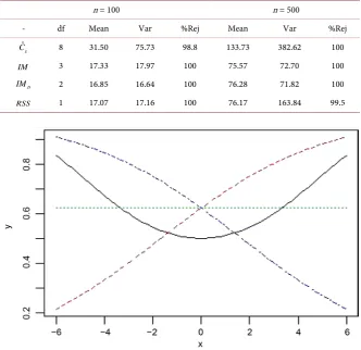
In Figure 1, we plot π vs x and we show the true model (continues line).

If we fit π =expit

(

α β+ x

)

, these putative approximation are shown for β<0, 0

[image:10.595.207.540.270.592.2]

β > _and β =0 (dot and dash, dash and dot) line respectively.

Table 3. Results of N = 1000 simulation with sample size n = 100 and n = 500 under wrong model.

n = 100 n = 500

- df Mean Var %Rej Mean Var %Rej

ˆ

g

C 8 31.50 75.73 98.8 133.73 382.62 100

IM 3 17.33 17.97 100 75.57 72.70 100

D

IM 2 16.85 16.64 100 76.28 71.82 100

RSS 1 17.07 17.16 100 76.17 163.84 99.5

Figure 1. Plots of the different logistic model π_i given X~U

(

−6,6

)

.

5. Conclusion and Further Work

the power of goodness-of-fit tests, which related the Rss , Hosmer-Lemeshow,

IM and IMDIAG tests under correct and missing model. However, our results

about the asymptomatic distribution of goodness-of-fit tests show, various com-binations of behavior on the mean and variance of statistics, which, the asymp-totic distribution of statistics is Chi-square

χ

2

df. The results under correct mod-el show reasonable power for all methods, slightly larger variance found in case of Hosmer-Lemeshow test, and smaller variance under missing covariate model. As we know the goodness-of-fit statistics are distributed asymptotically as central χ2 _{distribution under} H

0 when the model is correctly specified, and is

non-central χ2 _under H

1 when the model mis-specificed. However, under

wrong model the results show strange behavior, which all the means and va-riances are not satisfy the assumption on asymptotic distribution

χ

2

df with men

df and variance 2df, also, it is appeared with high power. The problem means that in some circumstances properties of the distribution of the statistics of tests (e.g mean and variance) are far away from the properties of χ2 _{distribution. In}

fact, the interesting point here, some of goodness-of-fit tests seem affected by assumption on covariance matrix. So, many issues about the mean and variance of the asymptotic distribution of goodness-of-fit statistic should also be ex-amined.

References

[1] Nelder, J.A. and Wedderburn, R.W.M. (1972) Generalized Linear Models. Journal of the Royal Statistical Society, Series A, 135, 370-384.

https://doi.org/10.2307/2344614

[2] Dobson, A. (1990) An Introduction to Generalized Linear Models. Chapman and Hall, London.

[3] Kleinbaum, D.G. (1994) Logistic Regression A Self-Learning Text. Springer-Verlag, New York.https://doi.org/10.1007/978-1-4757-4108-7

[4] Hosmer, D.W. and Lemeshow, S. (2000)Applied Logistic Regression. Wily, Chiche-ster.https://doi.org/10.1002/0471722146

[5] Hosmer, D., Lemeshow, S. and Sturdivant, R.X. (2013)Applied Logistic Regression. 3rd Edition, Wily, Chichester.https://doi.org/10.1002/9781118548387

[6] Hilbe, J.M. (2009) Logistic Regression Model.Chapman and Hall, New York. [7] Dobson, A.J. and Barnett, A.G. (2008) An Introduction to Generalized Linear

Mod-els. 3rd Edition, Chapman and Hall, New York.

[8] Kuss, O. (2002) Global Goodness-of-Fit Tests in Logistic Regression with Sparse Data. Statistics in Medicine, 21, 3789-3801.https://doi.org/10.1002/sim.1421

[9] Hosmer, D.W., Hosmer, T. and Lemeshow, S. (1980) A Goodness-of-Fit Tests for the Multiple Logistic Regression Model. Communications in Statistics, 10, 1043- 1069.https://doi.org/10.1080/03610928008827941

[10] Lemeshow, S. and Hosmer, D.W. (1982).A Review of Goodness of Fit Statistics for Use in the Development of Logistic Regression Models. American Journal of Epi-demiology, 115, 92-106.https://doi.org/10.1093/oxfordjournals.aje.a113284

https://doi.org/10.1002/(SICI)1097-0258(19970515)16:9<965::AID-SIM509>3.0.CO; 2-O

[12] Brown, C.C. (1982) On A Goodness of Fit Test for the Logistic Model Based on Score Statistics. Communications in Statistics Theory and Methods, 10, 1097-1105. https://doi.org/10.1080/03610928208828295

[13] McCullagh, P. and Nelder, J.A. (1989) Linear Models. 2nd Edition, Chapman and Hall, London.

[14] Copas, J.B. (1989) Testing for Neglected Heterogeneity. Econometrica, 52, 865-872. [15] Cox, D.R. and Snell, E.J. (1989) Analysis of Binary Data. 2nd Edition, Chapman and

Hall/CRC, London.

[16] Nagelkerke, N.D. (1991) A Note on a General Definition of the Coefficient of De-termination. Biometrika, 3, 691-692.https://doi.org/10.1093/biomet/78.3.691

[17] White, H. (1982) Maximum Likelihood Estimation of Misspecified Models. Eco-nometrica, 50, 1-25.https://doi.org/10.2307/1912526

[18] Lancaster, T. (1984) Covariance Matrix of the Information Matrix Test. Econome-trica, 4, 1051-1053.https://doi.org/10.2307/1911198

[19] Newey, W.K. (1984) Maximum Likelihood Specification Testing and Conditional Moment Test. Econometrica, 53, 1047-1070.

[20] Davidson, R. and Mackinnon, J.G. (1984) Convenient Specification Tests for Logit and Probit Models. Journal of Econometrics, 25, 241-262.

[21] Orme, C. (1988) The Calculation of the Information Matrix Test for Binary Data Models. EconPapers, 56, 370-376.

https://doi.org/10.1111/j.1467-9957.1988.tb01339.x

[22] Chesher, A. (1984) Unweighted Sum of Squares Test for Proportions. Econometri-ca, 38, 71-80.

Submit or recommend next manuscript to SCIRP and we will provide best service for you:

Accepting pre-submission inquiries through Email, Facebook, LinkedIn, Twitter, etc. A wide selection of journals (inclusive of 9 subjects, more than 200 journals)

Providing 24-hour high-quality service User-friendly online submission system Fair and swift peer-review system

Efficient typesetting and proofreading procedure

Display of the result of downloads and visits, as well as the number of cited articles Maximum dissemination of your research work

Submit your manuscript at: http://papersubmission.scirp.org/