Munich Personal RePEc Archive
A reconciliation of time preference
elicitation methods
Drichoutis, Andreas and Nayga, Rodolfo
University of Ioannina, University of Arkansas
19 April 2013
Online at
https://mpra.ub.uni-muenchen.de/46916/
A reconciliation of time preference elicitation methods
∗
Andreas C. Drichoutis
†1and Rodolfo M. Nayga, Jr.
‡21
University of Ioannina
2
University of Arkansas & Norwegian Agricultural Economics Research
Institute & Korea University
First Draft: April 19, 2013
This Version: May 12, 2013
Abstract
We reconcile findings from the Multiple Price List method (Andersen et al., 2008) and the Convex Time Budget method (Andreoni and Sprenger, 2012a) that seem to have generated a heated debate in the time preference literature. Specifically, we discuss the claims of Andreoni and Sprenger (2012b) that “risk preferences are not time preferences” and assert that this may have been premature given that subsequent findings from replication and extension studies refute their basic conjecture while another study offers an alternative explanation for their results (Andersen et al., 2011a). Although the CTB seems to perform better than the MPL method in terms of predictive validity, we also discuss recent econometric issues that question the validity of claims resulting from analysis of CTB data. We also raise an issue with non-EUT explanations of Andreoni and Sprenger’s (2012b) results, since the payment mechanism is not incentive compatible if the isolation assumption is not invoked.
Keywords: Intertemporal choice; discounting; curvature; convex time budget; risk; multiple price list.
JEL Classification Numbers: C91; D81; D91.
∗We would like to thank Stephen Cheung, Thomas Epper, Glenn Harrison, Michael Kuhn, Jayson Lusk
and Songfa Zhong for helpful comments and suggestions.
†Lecturer, Department of Economics, University of Ioannina, University campus, 45110, Greece, e-mail:
‡Professor and Tyson Endowed Chair, Department of Agricultural Economics & Agribusiness, Division
1
Introduction
Economic issues almost always involve the element of time and therefore, estimating time preferences is of paramount importance. Researchers have extensively relied on the use of the multiple price list format (MPL) that asks subjects to choose between time-dated payoffs, as a tool for inferring time preferences.
A major contribution in this line of research has been a method that relaxes the assump-tion of a linear utility funcassump-tion by inferring a subject’s curvature of the utility funcassump-tion from risk preferences (Andersen et al., 2008). In this (double) MPL method, the researcher ad-ministers both time and risk price lists and then jointly estimates risk and time preferences.1
Results from Andersen et al. (2008) generally show that if one does not take into account the curvature of the utility function, discount rates are upward biased.2
Another method that has recently garnered increasing attention (as judged by the number of subsequent replications and comments that have appeared in a relatively short amount of time) is the Convex Time Budget (CTB) method by Andreoni and Sprenger (2012a). In CTB, subjects are offered the possibility of intertemporally allocating their experimental budget between sooner and later payoffs instead of inferring the curvature of the utility function from risk preferences.3
Thus, by varying the interest rate and observing allocations, a researcher can infer the curvature of the utility function. In one sense, the CTB relaxes the constraint in Andersen et al. (2008) that only allows for corner allocations; that is, subjects can only choose between sooner and later payoffs (but not a mixture).
In a related paper, Andreoni and Sprenger (2012b) used the CTB method to make a claim that has caused a debate in the literature: “risk preferences are not time preferences”. They manipulated risk in intertemporal allocations and found that common ratio predictions of certain and risky outcomes are violated. The direct implication of this finding is that different utility functions might apply for time and risk. Since the publication of this paper, there has been a surge of related papers that tried to address the various issues with the CTB method (Cheung, 2012; Epper and Fehr-Duda, 2013a; Andreoni et al., 2013; Miao and Zhong, 2012).
1
Albeit nothing in this joint estimation approach requires that one uses MPL tasks. For example, subjects may presented with each choice on a separate screen as in Andersen et al. (2011b). The expression ‘MPL’ has been attached, perhaps abusively, to presentation methods of choices that resemble nothing close to price lists.
2
The issue of upward biased discount rate estimates in case of a concave utility function has been brought up in the review of Frederick et al. (2002). One of the techniques they suggest that would take into account the curvature of the utility function, is to “...separately elicit the utility function for the good in question, and then use that function to transform outcome amounts into utility amounts, from which utility discount rates could be computed”. They cite Chapman (1996) as the first study that attempted to do exactly this.
3
Given the importance of the topic, our purpose in this paper is to arbitrate the debate regarding elicitation of time preferences using the MPL and CTB methods. In the next sections, we first briefly discuss the MPL and CTB methods to set the stage and then review the issues raised with the CTB. We next discuss an alternative explanation by Andersen et al. (2011a) in relation to the claim that risk and time are mapped with different utility functions and a subsequent study by Andreoni et al. (2013) that compares the predictive validity of MPL and CTB. We then discuss some econometric issues on how one goes about estimating preference parameters from CTB data and raise the issue of the random lottery incentive mechanism that applies to all of the above cited studies. We conclude with our thoughts on the issues discussed herein, in the last section.
2
The MPL elicitation method
Andersen et al. (2008) separately administered multiple price lists of (riskless) temporal income streams (the time preference task) and (atemporal) multiple price lists of lotteries (the risk preference elicitation task).4
Typically, the time preference task is similar in spirit to Coller and Williams (1999) and the risk preference task is based on Holt and Laury (2002).5
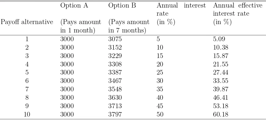
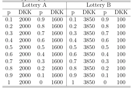
Table 1 and Table 2 show typical payoff tables shown to subjects in Andersen et al. (2008) where amounts are in Danish kroner.
In the time preference task, subjects are typically confronted with payoff tables similar to Table 1 and they make choices from several tables that have different time horizons. In Table 1, option A offers 3000 DKK in 1 month and option B offers 3000 DKK +x DKK in 7 months, where x ranges from annual interests rates of 5% to 50% on the principal of 3000 DKK. The table may or may not include the annual and annual effective interest rates that supposedly facilitates comparisons between lab and field investments.6
The tasks may
4
Andersen et al. (2006) note that Binswanger (1980) was the first experimental economist that used a MPL structure to elicit risk attitudes with real payoffs and Coller and Williams (1999) the first to have used a MPL format to elicit discount rates.
5
See also Takeuchi (2011) where subjects are asked to state i) their longest acceptable delay that makes two payment options at different points in time the same and ii) the lowest acceptable odds of winning the lottery for $y versus a sure amount of $x. Incentive compatibility is enforced through a BeckerDeGroot-Marschak mechanism (Becker et al., 1964).
6
provide two future income options or one instant and one future option.7
Table 1: Typical payoff matrix in the time preference task showing a 6 month horizon and one month front end delay
Option A Option B Annual interest rate
Annual effective interest rate Payoff alternative (Pays amount
in 1 month)
(Pays amount in 7 months)
(in %) (in %)
1 3000 3075 5 5.09
2 3000 3152 10 10.38
3 3000 3229 15 15.87
4 3000 3308 20 21.55
5 3000 3387 25 27.44
6 3000 3467 30 33.55
7 3000 3548 35 39.87
8 3000 3630 40 46.41
9 3000 3713 45 53.18
10 3000 3797 50 60.18
In the risk preference task, each subject is presented with a table of choices between two lotteries, A or B as illustrated in Table 2. In the first row the subject is asked to make a choice between lottery A, which offers a 10% chance of receiving 2000 DKK and a 90% chance of receiving 1600 DKK, and lottery B, which offers a 10% chance of receiving 3850 DKK and a 90% chance of receiving 100 DKK. The expected value of lottery A is 1640 DKK while for lottery B it is 475 DKK, which results in a difference of 1170 DKK between the expected values of the lotteries. Proceeding down the table to the last row, the expected values of the lotteries increase but more so for lottery B. Typically, subjects make choices from several tables where payoffs are scaled up. 8
(1999) design do not find evidence for hyperbolic discounting. More recent studies, however, that allow more than one data generating processes to explain discounting behavior, have found that observed choices are consistent with roughly one-half of the subjects using exponential discounting and one-half using quasi-hyperbolic discounting (Coller et al., 2012).
7
Using a front end delay (FED) on both sooner and later options has some advantages: first it avoids the passion for the present that decision makers exhibit when offered monetary amounts today or in the future and second, it allows the researcher to equalize the credibility of future payments. A third advantage is that it holds the transaction costs of future options constant in case these are not negligible (see for example the discussion in Coller and Williams, 1999). If ones decides not to use a FED, then extra care is needed in order to equalize transaction costs across all time periods, including physical costs and confidence. Andreoni and Sprenger (2012a) describe six specific measures to equate transaction costs and ensure payment reliablity. This is a very important step since there are some indications in the relevant literature that when transaction costs and payment risk are closely controlled, there is virtually no evidence of present bias (e.g., Andreoni et al., 2013).
8
Table 2: Typical payoff matrix in the risk preference task Lottery A Lottery B
p DKK p DKK p DKK p DKK 0.1 2000 0.9 1600 0.1 3850 0.9 100 0.2 2000 0.8 1600 0.2 3850 0.8 100 0.3 2000 0.7 1600 0.3 3850 0.7 100 0.4 2000 0.6 1600 0.4 3850 0.6 100 0.5 2000 0.5 1600 0.5 3850 0.5 100 0.6 2000 0.4 1600 0.6 3850 0.4 100 0.7 2000 0.3 1600 0.7 3850 0.3 100 0.8 2000 0.2 1600 0.8 3850 0.2 100 0.9 2000 0.1 1600 0.9 3850 0.1 100 1 2000 0 1600 1 3850 0 100
The result from Andersen et al. (2008) basically boils down to this: if one assumes that utility is linear in experimental payoffs when it is truly concave, then the estimated discount rates will be significantly biased upwards. Several studies since then have adopted a risk preference elicitation task as a complement to time preference elicitation as a necessary condition for capturing the concavity of utility functions and eliciting unbiased estimates of time preferences.9
3
The CTB elicitation method and a critique to MPL
The motivation for the Convex Time Budget (CTB) method of Andreoni and Sprenger (2012a) was to overcome a restriction of the MPL approach. Subjects that undertake the MPL time preference task are, by construction, restricted in choosing between corner allo-cations i.e., they can only choose a sooner amount X or a later amount Y. Thus, their in-tertemporal choice set is {(X,0),(0, Y)}. This choice set is then considered restrictive since if individuals have convex preferences in the sooner/later space, they will prefer interior so-lutions. Therefore, if researchers really want to identify convex preferences, then they should allow any choice along the intertemporal budget constraint connecting {(X,0),(0, Y)}.10
to scale up payoffs to allow for a wider range of dollar amounts, providing more information on the shape of the utility function. Alternatively, one may want to hold probabilities constant and vary the dollar amounts (Drichoutis and Lusk, 2012; Bosch-Dom`enech and Silvestre, 2012).
9
The interaction of risk and time preferences by the utility function is one of the many complex interac-tions between behavior under risk and behavior over time. Epper and Fehr-Duda (2013b) discuss a number of interaction effects between risk and time and attempt to rationalize the mounting empirical evidence within a single theoretical framework.
10
Andreoni and Sprenger (2012a) develop a single task to capture both discounting and concavity of the utility function by allowing subjects in each choice to choose a portfolio of sooner payoffs and later payoffs. In each CTB question, subjects are given a budget of 100 tokens which they have to allocate between a sooner and a later date. For example, in their “Sample Decision Screen” (Figure 1, pp.3340) the first choice is between an exchange rate of $0.20 per token on a sooner date (which amounts to $20 if all tokens are allocated to the sooner option) and $0.20 per token on a later date. The second choice is between an exchange rate of $0.19 on the same sooner date and $0.20 on the same later date. The later date exchange rate is in most cases kept constant at $0.20 and the sooner exchange rate was varied from $0.10 to $0.20.
For each choice (subjects faced 45 allocation problems), the subject decides on which fraction xof their 100 tokens is allocated to the sooner option and what fraction of 100−x
is allocated to the later option. In the first choice in their example, the allocation of 83 tokens to the sooner exchange rate of $0.20 and 17 tokens to the later $0.20 exchange rate amounts to $16.60 (83×0.20) and $3.40 (17×0.20) to the sooner and later date, respectively. Subjects were free to allocate either all tokens to the sooner option, all tokens to the later option or decide over an interior solution. In this sense, the CTB task allows more flexibility than the MPL task of Andersen et al. (2008) since it does not constrain subjects’ behavior to corner solutions.
Results from Andreoni and Sprenger (2012a) show that in aggregate, 37.1% of subjects select only corner solutions in the 45 convex budget sets. For the remaining 62.9% of the subjects, an average of around 50% of the choices are found at the corners, in any given decision. Put it otherwise, 70% of all choices were found at the extremes. Second, they estimate less curvature of the utility function as compared to the curvature elicited under a MPL. They do find, however, that the discount rates elicited with the MPL correlate well with the CTB estimates.
The basic design of Andreoni and Sprenger (2012a) was further utilized in Andreoni and Sprenger (2012b) to back up their claim that “risk preferences are not time prefer-ences”, which simply says that there are different utility functions under risk and under certainty. Andreoni and Sprenger (2012b) modified their basic design by allowing sooner payoffs and later payoffs to be realized with different independent probabilities, let’s call it
p1 andp2 respectively. Andreoni and Sprenger (2012b) implemented six different treatments
(p1, p2) ∈ {(1,1),(0.5,0.5),(0.5,0.4),(0.4,0.5),(1,0.8),(0.8,1)} where the (1,1) treatment
was the design in Andreoni and Sprenger (2012a). For the rest of the treatments, Andreoni and Sprenger (2012b) realized the sooner and later CTB payments using two independent
lotteries. The independent draw of lotteries is important since the criticism that is laid out in the next section hinges upon this design issue.
Andreoni and Sprenger (2012b) compared the certain treatment (1,1) to the one in which both payments are received with 50% probability and found that in the risky condition, subjects followed a more balanced allocation between sooner and later payments. The impli-cation is that different utility functions govern risk and time. This contrasts with Andersen et al. (2008) which assumed that only one utility function governs risk and time. In fact, since Andreoni and Sprenger (2012b) found that the utility function is more concave under risk than certainty, the MPL method would overcorrect for the utility curvature in discounting under certainty, which would result in much lower estimated discount rates.11
4
A debate over “risk preferences are not time
prefer-ences”
The methods and some claims in Andreoni and Sprenger (2012b) have resulted in a heated debate in the time preference literature. In this section we review some counter argu-ments and results from replication and extension experiargu-ments that scrutinized the findings in Andreoni and Sprenger (2012b).
Cheung (2012) scrutinized a procedural aspect of the CTB design which concerns the two
independent draws of lotteries for realizing the sooner and later payments. More specifically, he argued that subjects in the Andreoni and Sprenger (2012b) experiments could spread the risks by choosing mixtures of the two payments, while the corner allocation payments depend on just one lottery. He refered to this as a motive for “intertemporal diversification” that could provide an alternative explanation for Andreoni and Sprenger’s (2012b) findings that subjects prefer more balanced allocations between sooner and later payments under risk.
Cheung (2012) conducted a MPL and a CTB experiment. In the MPL experiment, he elicited both risk and time preferences using the procedures in Andersen et al. (2008) and added a treatment where discounting MPLs are received with a 50% probability. This experiment is basically a replication of Andreoni and Sprenger’s (2012b) main treat-ment {(1,1),(0.5,0.5)} in an MPL context. In the CTB experiment, he replicated the
{(1,1),(0.5,0.5)}treatments of Andreoni and Sprenger (2012b) and added a third treatment
11
where the sooner and later payoff were realized by a single lottery. In this new treatment, risks over sooner and later payments are perfectly correlated and thus precludes subjects from spreading their risks.
His results show no difference between the certainty and risk conditions in the MPLs. Cheung (2012) gave two explanations for this result: i) the MPL instrument may not be appropriately tailored to pick up differences in preferences that are detected by a CTB,12
and ii) subjects are not able to intertemporally diversify since the payment is determined by a single lottery. His CTB results show that once the opportunity for subjects to intertemporally diversify is taken away, the effect in Andreoni and Sprenger (2012b) remains, although it is reduced by one-half. Even though the difference between independent and correlated risks can be explained by concavity of intertemporal utility (captured by “correlation aversion” in Andersen et al., 2011a), there was still a residual difference about half in size as compared to when two independent lotteries were used. Thus, the conjecture of Andreoni and Sprenger (2012b) is not completely ruled out as a candidate explanation.
Miao and Zhong (2012) did an additional CTB treatment where there is a 50% chance that the sooner payment will be received, otherwise the later payment will be received.13
They replicated the finding from Andreoni and Sprenger (2012b) and Cheung (2012); in the (independent) risky condition: subjects followed a more balanced allocation between sooner and later payments as compared to the certain treatment. However, their “positive” treatment (which is the same as the “correlated” treatment that Cheung (2012) added to take away the opportunity that subjects intertemporally diversify) exhibited no difference with the certain treatment. This is in contrast to Cheung (2012) which reported that in his uncorrelated treatment the effect remained although reduced at half. Thus, the result from Miao and Zhong (2012) seems to refute the conjecture of Andreoni and Sprenger (2012b) in favor of an intertemporal diversification explanation. Although Miao and Zhong (2012) did not motivate the use of the “negative” treatment, they found that it generates similar intertemporal diversification as the “uncorrelated” treatment (we discuss the explanation provided by Epper and Fehr-Duda (2013a) momentarily). Note that the uncorrelated treat-ment corresponds to the original (0.5,0.5) treattreat-ment of Andreoni and Sprenger (2012b).
12
Note, that this claim is not explained in Cheung (2012) which may have prompted Harrison et al. (2013) to extensively argue in favor of the Binary Choice (BC) format of MPLs as compared to CTB.
13
Thus, Miao and Zhong (2012) conducted: i) a certain treatment (1,1), ii) a treatment where lotteries
Epper and Fehr-Duda (2013a) took on a claim of Andreoni and Sprenger (2012b) that non-EUT theories, such as prospect theory, cannot provide a unified account for the results they observed. When Andreoni and Sprenger (2012b) compared the (1,1) and (0.5,0.5) allo-cations, they observed that at the lowest interest rate, allocations are substantially higher in the (1,1) treatment, but as the interest rate increases, (1,1) allocations drop, crossing over the graph of the (0.5,0.5) treatment (Figure 2, pp.3367). Note that this finding emerges in the replication of the CTB experiments by Cheung (2012) and Miao and Zhong (2012). Andreoni and Sprenger (2012b) then claimed that this crossover in behavior cannot be ex-plained by probability weighting. When they compared treatments with differential risk but common ratios of probabilities (i.e, the {(1,0.8),(0.5,0.4)} and the {(0.8,1),(0.4,0.5)}
treatments), Andreoni and Sprenger (2012b) found that subjects exhibit allocations with a preference for certain payments relative to common ratio counterparts, regardless of whether the certain payment is sooner or later. These last findings can be explained by probabil-ity weighting which leads Andreoni and Sprenger (2012b) to note that “recognizing that violations correlate highly across contexts that can and cannot be explained by probability weighting suggests that prospect theory cannot provide a unified account for the data”.
Epper and Fehr-Duda (2013a) went on and assumed that subjects have Rank Dependent Utility (RDU) preferences. They showed that when the interest rateris relatively small, the discounted utility of sooner consumption will be greater than the discounted utility of later consumption. However, with rising interest rates, late consumption becomes increasingly attractive, which will lead to a change in the rank order of the discounted utilities. Thus, Epper and Fehr-Duda (2013a) rationalized the cross-over observation as the mechanics of decision weights, which is consistent with hedging behavior generated by the portfolio aspect of the risk environment. Epper and Fehr-Duda (2013a) also explained the difference in the “positive” and “negative” treatments of Miao and Zhong (2012) as consistent with RDU. Since in the “negative” treatment either the sooner or the later payment is realized (but not both) while in the “positive” treatment both payments are realized with a single draw, hedging opportunities can be present in the former but not in the latter.
5
Different utility functions or just “correlation
aver-sion”?
then we can write the intertemporal utility function as:
U(x, y) =
1 (1 +δ)t
x1−r
1−r +
1 (1 +δ)t+κ
y1−r
1−r
1−η,
1−η (1)
where δ is the exponential discount rate, x and y are money flows at time periods t and
t+κ respectively, r is the atemporal CRRA coefficient and η is the intertemporal CRRA coefficient. In (1), if we assume thatη= 0, that is, if we impose intertemporal risk neutrality, then we are back to assuming additive preferences over the time-dated money flows. This is the implicit assumption in all of the older literature, including Andersen et al. (2008). Note that the intertemporal risk type of the subject does not constrain the atemporal risk type. That is, the individual can be intertemporal risk averse (or “correlation averse”) and at the same time exhibit atemporal risk seeking, atemporal risk loving, or atemporal risk neutrality.
Correlation aversion is important because it directly questions the “risk preferences are not time preferences” claim of Andreoni and Sprenger (2012b) on a theoretical matter. Specifically, Andersen et al. (2011a) argued that when comparing behavior between subjects making choices over time-dated payoffs that are certain and subjects making choices over time-dated payoffs that are risky, one would indeed expect to observe different behavior. However, this behavior is evidence of correlation aversion (the name was coined by Epstein and Tanny (1980)) and does not necessarily mean that the utility functions of risk and time are different.14
Andersen et al. (2011a) argued that in the risky treatment of Andreoni and Sprenger (2012b), correlation aversion can affect subjects’ choices while in the certain treat-ment, correlation aversion can play no role. Although they did not rule out the hypothesis of different utility functions for risk and time, Andersen et al. (2011a) argued that there is a simpler solution at play which Andreoni and Sprenger (2012b) did not consider at all. These arguments for correlation aversion are made in passing in Andersen et al. (2011a) with respect to Andreoni and Sprenger (2012b), but are more thoroughly explained in Harrison et al. (2013).
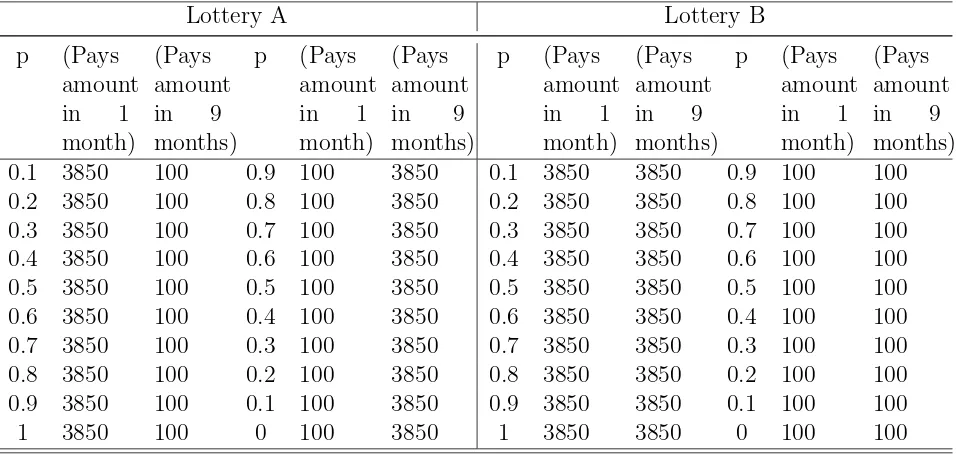
To elicit preferences, Andersen et al. (2011a) included one extra task. They used a time preference task as in Table 1, an atemporal risk preference task as in Table 2, and an intertemporal risk preference task as shown in Table 3. The rationale is that if you want to elicit intertemporal risk attitudes, you have to ask subjects to make choices over risky outcomes that are paid at different points in time.15
In the example shown in Table 3 (taken
14
Recall that Andreoni and Sprenger (2012b) found that when time-dated payoffs are certain, most allocations are at the corners (note that a MPL forces corner allocations) while when time-dated payoffs are risky, then subjects pick interior solutions more often.
15
from Andersen et al. (2011a)), lottery A gives the individual a 10% chance of receiving 3850 DKK in 1 month and 100 DKK in 9 months and a 90% chance of receiving 100 DKK in 1 month and 3850 DKK in 9 months. Lottery B gives the individual a 10% chance of receiving 3850 DKK in 1 month and 3850 DKK in 9 months and a 90% chance of receiving 100 DKK in one month and 100 DKK in 9 months. As one proceeds down the table the probability increases by 0.1 until the 10th row, where choices are then between certain outcomes.
Table 3: Typical payoff matrix in the intertemporal risk preference task showing an 8 month horizon and one month front end delay
Lottery A Lottery B
p (Pays amount in 1 month) (Pays amount in 9 months) p (Pays amount in 1 month) (Pays amount in 9 months) p (Pays amount in 1 month) (Pays amount in 9 months) p (Pays amount in 1 month) (Pays amount in 9 months) 0.1 3850 100 0.9 100 3850 0.1 3850 3850 0.9 100 100 0.2 3850 100 0.8 100 3850 0.2 3850 3850 0.8 100 100 0.3 3850 100 0.7 100 3850 0.3 3850 3850 0.7 100 100 0.4 3850 100 0.6 100 3850 0.4 3850 3850 0.6 100 100 0.5 3850 100 0.5 100 3850 0.5 3850 3850 0.5 100 100 0.6 3850 100 0.4 100 3850 0.6 3850 3850 0.4 100 100 0.7 3850 100 0.3 100 3850 0.7 3850 3850 0.3 100 100 0.8 3850 100 0.2 100 3850 0.8 3850 3850 0.2 100 100 0.9 3850 100 0.1 100 3850 0.9 3850 3850 0.1 100 100 1 3850 100 0 100 3850 1 3850 3850 0 100 100
The main result of Andersen et al. (2011a) was that subjects exhibit intertemporal risk aversion as well as atemporal risk aversion. They also found that intertemporal risk aversion accounts for a substantial amount of the estimated risk premium. Based on these results, Andersen et al. (2011a) point that the claim of AS that “risk preferences are not time preferences” can be restated more carefully as “atemporal risk aversion is not the same as intertemporal risk aversion”.
6
Further contributions to the debate: CTB vs. MPL
A subsequent paper by Andreoni et al. (2013) explored the predictive validity of the CTB method (Andreoni and Sprenger, 2012a,b) and the double MPL (Andersen et al., 2008), where double refers to the fact that one needs a risk MPL and a time MPL to identify the curvature of the utility function. Although predictive validity is an important benchmark
that can be used to compare methods, it does not address the points raised in Andersen et al. (2011a) regarding correlation aversion. Thus, Andreoni et al. (2013) is all about comparing two time preference elicitation methods over certainty but not over intertemporal risky options.
Andreoni et al. (2013) elicited risk and time preferences using the standard method of Andersen et al. (2008). They used two MPL structures, one that asks subjects to choose between intertemporal choices (similar to Table 1) and one that asks subjects to choose between lotteries (similar to Table 2). Their experiment utilized a within-subjects design so that the same subjects also participated in a CTB task, which was relatively different in terms of the decision environment from that used in Andreoni and Sprenger (2012a,b). In particular, instead of allowing individuals to make continuum intertemporal allocations, they discretized the possible allocations to six options so that the format more closely resembles the MPL format. The CTB task implemented was certain, that is, it corresponded to the (1,1) treatment in Andreoni and Sprenger (2012b).
At the end of the CTB and double MPL tasks, one choice was randomly chosen as binding. Subjects were subsequently asked about their willingness-to-accept (WTA) in their sooner payment to forego a claim to an additional $25 in their later payment. To make the task incentive compatible, the BDM mechanism was implemented (Becker et al., 1964). In addition, two hypothetical measures were elicited. They asked subjects to indicate which dollar amount of money today would make them indifferent to $20 in one month and which amount of money in one month would make them indifferent to $20 today.
The results showed two things. First, the double MPL (DMPL) results in a much lower discount rate (47.2% vs. 74.1%) although the estimate lies within the 95% confidence interval of the CTB estimate, which had a wide standard error of 39%.16
Second, the DMPL shows significant curvature for the utility function (they estimate an α = 0.55) although it is estimated to be almost linear using the CTB data (α = 0.95). This very high curvature of the utility function is the reason why the discount rate is much lower in the DMPL.
To assess the predictive validity of the two methods, they used in- and out-of-sample fit criteria. Andreoni et al. (2013) found that the DMPL performs slightly better in-sample. For example, in-sample individual MPL estimates predict 89% of MPL choices correctly while they predict only 75% correctly for CTB. Moreover, individual CTB estimates predict 86% of MPL choices correctly while individual MPL estimates correctly predict only 16% of CTB choices.
16
Andreoni et al. (2013) then compared the out-of-sample prediction on the amount sub-jects were willing to accept in their sooner payment to forgo $25 in the later payment as well as on the two hypothetical questions. In general, they found that while both methods are off at the aggregate level, “DMPL predictions provide limited added predictive power beyond the CTB predictions”. Andreoni et al. (2013) claimed that the difference in the predictive validity of CTB and DMPL comes from the source of information for the utility function curvature (i.e., the CTB curvature is inferred by changing interest rates while the DMPL curvature is informed by risk preferences).
Given the discussion above, one can surmise that the issue of how to best infer the curva-ture of the utility function is of importance to this literacurva-ture. It is not clear however why the DMPL results in a much higher curvature when in the CTB task, 88% of total allocations are at one of the two budget corners, implying a linear utility function. Nevertheless, much of the comparisons laid out above depend on the use of specific econometric methods for inferring preference parameters. There is one issue remaining on how one goes about esti-mating preference parameters from CTB data that was recently brought up in this debate. We discuss this in the next section.
7
The econometrics of CTB data
In a subsequent comment of the CTB paper (Andreoni and Sprenger, 2012a), Harrison et al. (2013) criticize the econometric techniques used by Andreoni and Sprenger (2012a). Their point is based on the fact that the vast majority of choices (70%) is at the extremes of sooner and later payoffs. Therefore, the distribution of the fraction allocated to sooner payoffs (which takes on values between 0 and 100) has massive spikes at 0 and at 100.
First, Harrison et al. (2013) point that when Andreoni and Sprenger (2012a) use non-linear least squares (NLS), they invite heteroskedasticity problems. This is because the error term wanders between ±∞, but the choice data are restricted to the [0, 100] interval. Second, Andreoni and Sprenger (2012a) focus on explaining the average portfolio allocation even though the average is nowhere close to their data and the vast majority of choices are found at corner allocations. This significantly affects prediction allocations which, as Harrison et al. (2013) show, lie to the interiors of the boundaries 0 and 100. The implication is that residuals from these estimations can highly reject the null of normality.
is zero or negative, ii) the choice will be 100 if the latent variable is 100 or greater and iii) the choice will be in the interval (0, 100) if the latent variable is (0, 100). Harrison et al. (2013) argue that given that the utility specification is defined only over money offered in the lab, the assumption of a latent variable below 0 or above 100 makes no theoretical sense. The Tobit specification is seen as an improvement since it can correctly account for the choices at 0 or 100, although it “...still fails to address the concern that the error term can imply theoretically incoherent values of the latent variable for all interior allocations.”
So how can one correctly model choices from CTB data? Harrison et al. (2013) propose that the most natural approach is to assume that subjects choose one of the 101 percentage point allocations between 0 and 100 and define a latent index:
∇U = expUτ/(expU0%+ expU1%+. . .+ expU100%) (2)
where U is the intertemporal utility function and τ indexes the specific choice that was observed. As such, equation (2) indexes a multinomial logit probability of observing the choice τ and can be estimated using familiar maximum likelihood methods. Harrison et al. (2013) estimate this model using data from Andreoni and Sprenger (2012a) and find results that imply a convex utility function, with a RRA estimate of -0.36 and a discount rate estimate of 60.1%. The striking result here is the finding of the existence of a convex utility function. As Harrison et al. (2013) note, this contrasts with the findings from the literature that generally reflects a concave utility functions.
Harrison et al. (2013) argue that the finding of a convex utility function is the result of estimating a structural model that focuses on the averages under the assumption of homo-geneous representative agents. As they argue, only a convex utility function can explain the choice pattern of extreme allocations. In fact, a concave utility function would predict all optimal choices into the interior, which is not consistent with the observed data.
8
Some further considerations: The random lottery
incentive mechanism
All the cited studies above refer, one way or another, to behavior that departs from expected utility.17
However, there may be a problem with results coming from designs that apply the random lottery incentive mechanism (RLIM) for non-EUT specifications (i.e., the fact that they randomly choose one of the choices for payout). Non-EUT specifications violate the independence axiom (IA) while a RLIM maintains that the axiom is valid for the task to be incentive compatible. This concern is not specific to the above cited studies but to the hundreds of studies that used the RLIM and introduced a theoretical confound when they set out to test non-EUT alternatives. Researchers have different views about this issue. For example, Wakker (2007) argued that this issue has unduly hindered many papers in the review process and that it is counter-productive to re-hash the issue each and every time.
The theoretical criticism of RLIM was first put forward by Holt (1986) who argued that if the IA of Expected Utility Theory is not satisfied, then the experiment might fail to elicit true preferences. The criticism was subsequently shown by Starmer and Sugden (1991), Cubitt et al. (2004) and Hey and Lee (2005) to have no empirical merit. The RLIM has since been used without second thought by many experimental economists.18
The random selection mechanism has been favored because it is known to avoid wealth and portfolio effects that arise with alternative payoff mechanisms such as if one decides to pay all decisions sequentially during the experiment or all decisions at the end of the experiment. However, the issue is still being debated and often, referees will invoke arguments along the lines of Holt (1986), which obviously prompted Hey and Lee (2005) to explicitly conclude that: “...experimenters can continue to use the random lottery incentive mechanism and that this paper can be used as a defence against referees who argue that the procedure is unsafe”.
In essence, researchers that use the RLIM under non-EUT specifications invoke the as-sumption of the isolation effect i.e., that a subject views each choice in an experiment as independent of other choices in the experiment. If the isolation assumption holds, then RLIM is incentive compatible even under non-EUT specifications. However, if the isolation effect does not hold, then there is no alternative for multi-decision experiments where behavior departs from EUT. The debate then boils down to an empirical question of whether the isolation effect holds or not.
As mentioned above, several studies have defended the validity of RLIM. Nevertheless, the issue has been re-opened recently by Cox et al. (2011), Harrison et al. (2012) and Harrison and Swarthout (2012). Cox et al. (2011) tested a one-task (OT) decision environment which is the only alternative payoff mechanism that is valid under any behavioral decision theory. In
17
Albeit, the correlation aversion explanation does not depend on the assumption of EUT or RDU. In addition, when Andersen et al. (2011a) allow for non-EUT preferences in their models they find this has no real impact on results.
18
OT, a subject makes only one choice and is paid for that choice. The mechanism comes with some caveats though. For example, it precludes within-subjects hypothesis tests since in such experiments a subject only makes one decision. Another assumption is therefore required pertaining to preferences across subjects being homogeneous. Harrison et al. (2012) pointed out that “...plausible estimates of the degree of heterogeneity in the typical population imply massive sample sizes for reasonable power, well beyond those of most experiments”. The implications for experimental practice, in terms of the cost of having much larger sample sizes coupled with the need to conduct high stakes experiments, are profound.
While Cox et al. (2011) presented evidence against the isolation effect and advocated the use of OT, they also noted that more systematic exploration is needed to answer the question of whether biases introduced into data by RLIM are insignificant in some (or most) contexts. Thus, while the jury is still out on this, we definitely need more studies that explore the degree of bias that occurs when RLIM is used in time preference elicitation. If the bias is significant, then claiming that non-EUT theories can explain any of the effects discussed in the previous sections would be a sign of bipolar behaviorism (Harrison and Swarthout, 2012).
9
Conclusion
In this paper, we tried to arbitrate findings from the MPL method (Andersen et al., 2008) and the CTB method (Andreoni and Sprenger, 2012a) that seem to have generated a heated debate in the time preference literature. Andreoni and Sprenger (2012b) presented some findings that challenged the notion that risk and time are mapped using the same utility function. However, their main conjecture seems to have been refuted partially (Cheung, 2012) or completely (Miao and Zhong, 2012) by subsequent replications and extensions. Andersen et al. (2011a) maintained that the results of Andreoni and Sprenger’s (2012b) could easily be explained by intertemporal risk aversion (correlation aversion) without having to resort to claiming that “risk preferences are not time preferencess”.
There is no question that the literature on how to best elicit time preferences is still evolving. The findings from Andreoni et al. (2013) require more thorough testing. For example, it would be important to decipher why the MPL and CTB methods provide different estimates as to the level of the curvature of the utility function since this has immense and direct implications for the estimation of discount rates. In that respect, we also need to take into serious account the econometric issues raised in Harrison et al. (2013).
References
Andersen, S., G. W. Harrison, M. Lau, and E. E. Rutstr¨om (2011a). Multiattribute utility
theory, intertemporal utility and correlation aversion. Center for the Economic Analysis
of Risk, Working Paper 2011-04, Robinson College of Business, Georgia State University.
Andersen, S., G. W. Harrison, M. I. Lau, and E. E. Rutstr¨om (2006). Elicitation using
multiple price list formats. Experimental Economics 9(4), 383–405.
Andersen, S., G. W. Harrison, M. I. Lau, and E. E. Rutstr¨om (2008). Eliciting risk and time
preferences. Econometrica 76(3), 583–618.
Andersen, S., G. W. Harrison, M. I. Lau, and E. E. Rutstr¨om (2011b). Discounting behavior:
A reconsideration. Center for the Economic Analysis of Risk, Working Paper 2011-03,
Robinson College of Business, Georgia State University.
Andreoni, J., M. A. Kuhn, and C. Sprenger (2013). On measuring time preferences. Working
paper, University of California at San Diego.
Andreoni, J. and C. Sprenger (2012a). Estimating time preferences from convex budgets.
The American Economic Review 102(7), 3333–56.
Andreoni, J. and C. Sprenger (2012b). Risk preferences are not time preferences. The
American Economic Review 102(7), 3357–3376.
Becker, G. M., M. H. Degroot, and J. Marschak (1964). Measuring utility by a single-response
sequential method. Behavioral Science 9(3), 226–232.
Binswanger, H. P. (1980). Attitudes toward risk: Experimental measurement in rural india.
American Journal of Agricultural Economics 62(3), 395–407.
Bosch-Dom`enech, A. and J. Silvestre (2012). Measuring risk aversion with lists: a new bias.
Chapman, G. B. (1996). Temporal discounting and utility for health and money. Journal of
Experimental Psychology: Learning, Memory, and Cognition 22(3), 771–91.
Cheung, S. L. (2012). Risk preferences are not time preferences: Comment. Institute for the
Study of Labor (IZA) Discussion Paper No 6762.
Coble, K. and J. Lusk (2010). At the nexus of risk and time preferences: An experimental
investigation. Journal of Risk and Uncertainty 41(1), 67–79.
Coller, M., G. W. Harrison, and E. E. Rutstr¨om (2012). Latent process heterogeneity in
discounting behavior. Oxford Economic Papers 64(2), 375–391.
Coller, M. and M. Williams (1999). Eliciting individual discount rates. Experimental
Eco-nomics 2(2), 107–127.
Conlisk, J. (1989). Three variants on the allais example. The American Economic
Re-view 79(3), 392–407.
Cox, J. C., V. Sadiraj, and U. Schmidt (2011). Paradoxes and mechanisms for choice under
risk.Center for the Economic Analysis of Risk, Working Paper 2011-12, Robinson College
of Business, Georgia State University.
Cubitt, R. P., A. Munro, and C. Starmer (2004). Testing explanations of preference reversal.
The Economic Journal 114(497), 709–726.
Cubitt, R. P. and D. Read (2007). Can intertemporal choice experiments elicit time
prefer-ences for consumption? Experimental Economics 10(4), 369–389.
Drichoutis, A. C. and J. L. Lusk (2012). What can multiple price lists really tell us about
risk preferences? Munich Personal RePEc Archive Paper No. 42128.
Epper, T. and H. Fehr-Duda (2013a). Balancing on a budget line: Comment on Andreoni
and Sprenger’s “Risk preferences are not time preferences”. Working paper, ETH Zurich
Epper, T. and H. Fehr-Duda (2013b). The missing link: Unifying risk taking and time
discounting. Working paper No. 96, Department of Economics, University of Zurich.
Epstein, L. G. and S. M. Tanny (1980). Increasing generalized correlation: A definition and
some economic consequences. The Canadian Journal of Economics 13(1), 16–34.
Frederick, S., G. Loewenstein, and T. O’Donoghue (2002). Time discounting and time
preference: A critical review. Journal of Economic Literature 40(2), 351–401.
Harrison, G. W., M. I. Lau, and E. E. Rutstr¨om (2013). Identifying time preferences with
experiments: Comment. Center for the Economic Analysis of Risk, Working Paper
2013-05, Robinson College of Business, Georgia State University.
Harrison, G. W., J. Martinez-Correa, and J. T. Swarthout (2012). Reduction of compound
lotteries with objective probabilities: Theory and evidence. Center for the Economic
Analysis of Risk, Working Paper 2012-05, Robinson College of Business, Georgia State
University.
Harrison, G. W. and J. T. Swarthout (2012). The independence axiom and the bipolar
behaviorist. Center for the Economic Analysis of Risk, Working Paper 2012-01, Robinson
College of Business, Georgia State University.
Hey, J. D. and J. Lee (2005). Do subjects separate (or are they sophisticated)? Experimental
Economics 8(3), 233–265.
Holt, C. A. (1986). Preference reversals and the independence axiom. The American
Eco-nomic Review 76(3), 508–515.
Holt, C. A. and S. K. Laury (2002). Risk aversion and incentive effects. The American
Economic Review 92(5), 1644–1655.
Kreps, D. M. and E. L. Porteus (1978). Temporal resolution of uncertainty and dynamic
Miao, B. and S. Zhong (2012). Separating risk preference and time preference. Working
paper, National University of Singapore.
Starmer, C. and R. Sugden (1991). Does the random-lottery incentive system elicit true
preferences? an experimental investigation. The American Economic Review 81(4), 971–
978.
Takeuchi, K. (2011). Non-parametric test of time consistency: Present bias and future bias.
Games and Economic Behavior 71(2), 456–478.
Wakker, P. P. (2007). Message to referees who want to embark on yet another discussion of
the random-lottery incentive system for individual choice. Available at http://people.