Variational Homotopy Perturbation Method for Solving Riccati Type Differential Problems

(1)

http://www.scirp.org/journal/am ISSN Online: 2152-7393

ISSN Print: 2152-7385

Variational Homotopy Perturbation Method for

Solving Riccati Type Differential Problems

Bothayna S. Kashkari, Sharefah Saleh

Department of Mathematics, Faculty of Sciences, King Abdulaziz University, Jeddah, Saudi Arabia

Abstract

In this paper, a Variational homotopy perturbation method is proposed to solve nonlinear Riccati differential equation. By combining the Variational Iteration Method and the Homotopy Perturbation Method, this technique possesses a fast convergence rate with high accuracy. The results reveal that the proposed method is very effective and simple.

Keywords

Riccati Equation, Homotopy Perturbation Method, Variational Iteration Method, Variational Homotopy Perturbation Method

1. Introduction

The Riccati equation plays a great role in blueprint and analysis the linear and nonlinear optimal control problems. Numerical Solution of this equation has been acquired by applying Adomian’s decomposition method [1], homotopy Analysis method HAM [2], variational iteration method VIM [3] and homotopy perturbation method HPM [4]. HPM introduced by He [5], it can solve a large class of nonlinear problems activity, accurately and easily.

The application of HPM on nonlinear problems has been implemented by scientists and engineers, because this method is to continuously deform a diffi-cult problem under study into a simple problem easy to solve. VIM proved by Ji- Huan He [5]. It is simple and powerful method for solving a broad type of non-linear Problem. It was shown that this method is operative and reliable analytic and numerical purposes. The method gives rapidly convergent successive ap-proximation of the exact solution if such solution existed.

The nonlinear Riccati differential equation [6] has following form

( )

( ) ( )

( )

2

, 0 0

L x A x u x B x u x C x x X

u α

= + + ≤ ≤

= (1)

How to cite this paper: Kashkari, B.S. and Saleh, S. (2017) Variational Homotopy Per- turbation Method for Solving Riccati Type Differential Problems. Applied Mathema- tics, 8, 893-900.

https://doi.org/10.4236/am.2017.87070 Received: May 26, 2017

Accepted: July 1, 2017 Published: July 4, 2017

http://creativecommons.org/licenses/by/4.0/

(2)

where d

d

L x

= or 22

d

dx , A x B x

( ) ( )

, and C x

( )

are continuous functions and α _{is an arbitrary constant.}

We organize the following paper as follows. In Section 2, we present the VIM, while in Section 3, we present the HPM. In Section 4, we apply the VHPM to solve quadratic Riccati equation. Moreover, we find solutions of some examples by VHPM in Section 5.

The results reveal that the proposed method is very effective and simple. We end this paper by conclusion that reveal that these methods are very effective and convenient for solving nonlinear Riccati equations.

2. Variational Iteration Method

To illustrate the basic concepts of the VIM we consider the following differential equation [7] [8]

( )

L u +N u = f x (2)

where L is a linear operator, N is a nonlinear operator, and f x

( )

is an

inho-mogeneous term. Then, we can construct the correct functional as follows

( ) ( )

( )

1 ₀ d

x

n n n n

u+ =u +

∫

λ ξ

L u +N u −f

ξ



ξ

(3)

where λ _{is a general Lagrangian multiplier defined as}_[9]

( ) ( )

₍

1

_{) (}

)

1

, , 1

1 !

m

x t x t m

m

λ − −

= − ≥

− (4)

And un are restricted variation which means δun=0. Consequently, the solution lim _n

n

u u

→∞

= _.

3. Homotopy Perturbation Method

To explain this method, we construct the following function [10]

( )

0,

A u − f x = x∈Ω (5)

With boundary condition

(

,

)

0,

B u u n∂ ∂ = x∈Γ (6)

where

A

is a general differential operator,

B

is a boundary operator, f x

( )

is a known analytical function. The operator

A

can be decomposed into two

operators

L

and N, where

L

is a linear operator and N is a nonlinear

operator.

By using the homotopy technique, we construct a homotopy

(

,

)

:

[ ]

0,1

u x p Ω× → which are satisfies

(

,

) (

1

) ( )

( )

0

( )

0

H u p = −p _L u −L u _+p L u_ +N u − f x _= (7)

or

(

,

)

( )

0

( )

0

( )

0

H u p =L u −L u +p L u_ +N u − f x _= (8)

(3)

solution of equation.

( )

0

L u +N u − f x = (9)

We have

( )

, 0

( )

0 0,

( )

,1

( )

0

H u =L u +L u = H u =A u − =f (10)

The solution can be written as a power series in p,

( )

2

0 1 2

1 lim

p

u x u u pu p u

→

= = + + +__.

4. Variational Homotopy Perturbation Method

In this section, we apply the VHPM to Riccati Equation (1), we start this method by applying HPM in Equation (8) on Equation (1), we get

( )

2

( )

0 0 0

n n n

Lu x −Lu x +p Lu_ x −A x u −B x u −C x _= (11)

Now we using correction functional in Equation (5) to get

( )

(

( )

2

( )

)

1 ₀ 0 0 d

x

n n n n n

u+ =u +

∫

λ ξ

Lu −Lu +p Lu −A

ξ

u −B

ξ

u −C

ξ



ξ

(12)

We can obtain

( )

2

( )

1 0 ₀ 0 n d

x

n n

u₊ =u +p

∫

λ ξ

_Lu −A

ξ

u −B

ξ

u −C

ξ

_

ξ

(13)

Now we can rewrite Equation (13) in the form

( )

0 0

0 0 0

d

x

n n

p u u p

λ ξ

Lu N p u C

ξ

∞ ∞

= =

  

= + _ _ − − __

 

 

∑

∫

∑

 (14)

As we see, the procedure is formulated by the coupling of VIM and HPM [11] [12] [13]. A comparison of like powers of p give solutions of various orders.

5. Numerical Examples

5.1. Example

Consider the following classical Riccati differential equation

( )

2

2 1

u x′ = − +u u+ (15)

With initial condition u

( )

0 =0.

For the above differential equation, the exact solution [14] is previously known to be

( )

1 2 1

1 2 tanh 2 log 2 2 1

u x = + _ x+ _ − __

+

 

  (16)

The Taylor expansion of u x

( )

about x=0 gives

( )

2 1 3 1 4 7 5 7 6 53 7

3 3 15 45 315

u x = +x x + x − x − x − x + x + (17)

Suppose that the initial approximation is u0=x.

To solve Equation (15), by the VHPM we substitution it in Equation (14)

2

0

0 0 0 0

2 d

x

n n n

p u u p p u p u

ξ

∞ ∞ ∞

= = =

 _ _ 

= − − +_ _ 

 

 

 

(4)

Here λ = −1.

By comparing the coefficient of like powers of p, we have

( ) ( )

(

)

( )

₍

₎

( )

(

)

0 0

1 2 2 3

1 ₀ 0 0

2 3 4 5

2 ₀ 1 0 1

3 2 4 5 6 7

3 ₀ 2 0 2 1

:

1

: 2 d

3

2 2 2

: 2 2 d

3 3 15

1 11 17 17

: 2 2 d

3 15 45 315

x x x

p u x

p u u u x x

p u u u u x x x

p u u u u u x x x x

ξ ξ ξ = = − − + = − = − − + = − + = − − + + = − + −

∫

 (19)

The other components of the VHPM can be determined in similar way. Final-ly, the approximate solution of Equation (15) is u=u0+ +u1 u2+u3+. Which

converge to the exact solution in Equation (16).

5.2. Example

Consider the following quadratic Riccati differential equation

( )

2 2 3

2ex 2e x ex ex

u x′ = − u + u+ − (20)

With initial condition u

( )

0 =1.

For the above differential equation, the exact solution [14] is previously known to be

( )

ex

u x = (21)

The Taylor expansion of u x

( )

about x=0 gives

( )

1 2 1 3 1 4 1 5 1 6 1 7

1

2 6 24 120 720 5040

u x = + +x x + x + x + x + x + x + (22)

Suppose that the initial approximation is u0= +x 1.

To solve Equation (20), by the VHPM we substitution it in Equation (14), then we get

( )

2

( )

0

0 0 0 0 0 0 0 0

2 2 3

1 2 d

! ! ! !

n n n

x n

n n n

n n n n n n n

p u u p p u p u

n n n n

ξ

_ξ

∞ ∞ ∞ ∞ ∞ ∞ ∞ = = = = = = =  _ _ _ _  = −  + _ _− _ _ + −         

∑

∫

∑

(23)

Here λ = −1.

( ) ( ) ( ) ( ) 0 0

1 2 3 4 5 6 7 8

1

9 10

2 5 6 7 8 9 10

2

3 5 6 7 8 9 10

3

: 1

1 1 1 1 49 37 1091

:

2 6 24 24 270 270 40320

247 1

45360 50400

1 5 13 23 19 3389

:

10 36 126 480 2592 302400

1 5 13 1 59 32119

:

20 72 252 120 1728 604800

p u x

p u x x x x x x x

x x

p u x x x x x x

= + = + + − − − − + − = + + + + − − = − − − − + +  +_  (24)

(5)

Final-ly, the approximate solution of Equation (20) is u=u0+ +u1 u2+u3+. Which

converge to the exact solution in Equation (21).

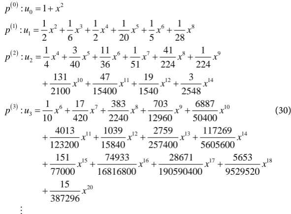
5.3. Example

Consider the Riccati Type Painleve’s First Transcendent equation [15]

( )

2

6 , 1

u x′′ = u +

µ

x

µ

= (25)

With initial conditions u

( )

0 =1,u′

( )

0 =0.

The above differential equation without known exactly solutions and we sup-pose that the initial approximation is 2

0 1

u = +x .

To solve Equation (25) by the VHPM, substitution it in Equation (14), then we get

( )

2

0

0 0 0

2 6 d

x

n n

p u u p

λ ξ

p u

ξ ξ

∞ ∞

= =

 _ _ 

= +  − _ _ − 

 

 

 

∑

∫

∑

(26)

In this example

λ

=

(

ξ

−x

)

.

( )

0 2

0

1 2 3 4 6

1

2 4 5 6 7 8 10

2

3 6 7 8 9 1

14

0 11

3

12

: 1

1 1 : 2

6 5

1 6 1 9 2 : 2

10 5 21 35 75 8 13 1877 11 11 17 :

5 105 1680 210 35 1925 254

5775 325

p u x

p u x x x x

p u x x x x x x

p u x x x x x

x

= +

= + + +

= + + + + +

+ +



(27)

The other components of the VHPM can be determined in similar way. Final-ly, the approximate solution of Equation (25) is u≈u0+ +u1 u2+u3+. In Ta-ble 1 we present the comparison between the approximate solution founded by VHPM with Truncated Taylor series(TTS) [16], and Rational approximation (RA) [17].

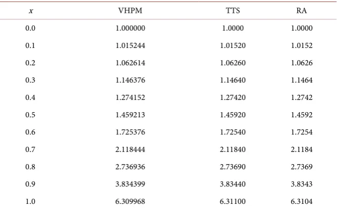
5.4. Example

Consider the Riccati Type Painleve’s Second Transcendent equation [15]

( )

₂ 3 _, ₁

u′′ x = u +xu+

µ µ

= (28)

With initial conditions u

( )

0 =1,u′

( )

0 =0.

The above differential equation without known exactly solutions and we sup-pose that the initial approximation is 2

0 1

u = +x .

To solve Equation (28) by the VHPM, substitution it in Equation (14), then we get

( )

3

0

0 0 0 0

1 2 d

x

n n n

p u u p

λ ξ

p u

ξ

p u

ξ

∞ ∞ ∞

= = =

 _ _ 

= +  − _ _ − 

 

 

 

(6)

[image:6.595.208.539.103.308.2]

Table 1. Comparison between the approximate solution 20 0

i i

u u

=

∑

with TTS and RA.

x VHPM TTS RA

0.0 1.000000 1.0000 1.0000

0.1 1.030471 1.030471 1.0305

0.2 1.126366 1.126366 1.1264

0.3 1.301454 1.301453 1.3015

0.4 1.583055 1.583054 1.5831

0.5 2.022763 2.022771 2.0228

0.6 2.721246 2.721242 2.7212

0.7 3.890893 3.890886 3.8909

0.8 6.038351 6.038340 6.0383

0.9 10.622497 10.622610 10.6223

1.0 23.363804 23.393600 23.3860

And we have

λ

=

(

ξ

−x

)

.

( )

0 2

0

1 2 3 4 5 6 8

1

2 4 5 6 7 8 9

2

1 11 12 14

6 7 8 9 10

1 0

1 3

3

47 19 3

15400 1540 2548

17 383 703 6887

10 420 2240 12960 5040

: 1

1 1 1 1 1 1

:

2 6 2 20 5 28

1 3 11 1 41 1

:

4 40 36 51 224 224

131 210

0 4013

12320 0

0 1 :

x

p u x

p u x x x x x x

x x

p u

x

x x x x x

x

+ + +

+ + + +

= +

= + + + + +

+

+ =

+ 12 13 14

15 16 17 18

20

1039 2759 117269

15840 257400 5605600

151 74933 28671 5653

77000 16816800 190590400 9529520 15

387296

x x x

x x x x

x

+ +

+ + + +

+



(30)

The other components of the VHPM can be determined in similar way. Final-ly, the approximate solution of Equation (28) is u≈u0+ +u1 u2+u3+ . In Table 2 we present the comparison between the approximate solution founded by VHPM with TTS [15], and RA [17].

6. Conclusion

[image:6.595.242.538.357.575.2]

(7)

[image:7.595.208.539.102.308.2]

Table 2. Comparison between the approximate solution 20 0

i i

u u

=

∑

_{with TTS and RA.}

x VHPM TTS RA

0.0 1.000000 1.0000 1.0000

0.1 1.015244 1.01520 1.0152

0.2 1.062614 1.06260 1.0626

0.3 1.146376 1.14640 1.1464

0.4 1.274152 1.27420 1.2742

0.5 1.459213 1.45920 1.4592

0.6 1.725376 1.72540 1.7254

0.7 2.118444 2.11840 2.1184

0.8 2.736936 2.73690 2.7369

0.9 3.834399 3.83440 3.8343

1.0 6.309968 6.31100 6.3104

comparison between the numerical results with TTS and RA in Problems 3 and 4 of validates the accuracy of the VHPM method for problems without known exactly solutions that have been advanced for solving Riccati equation shows that the new technique is reliable and powerful.

References

[1] Gbadamosi, B., Adebimpe, O., Akinola, E.I. and Olopade, I.A. (2012) Solving Ricca-ti EquaRicca-tion Using Adomian DecomposiRicca-tion Method. International Journal of Pure and Applied Mathematics, 78, 409-417.

[2] Tan, Y. and Abbasbandy, S. (2013) Homotopy Analysis Method for Quadratic Ric-cati Differential Equation. Communications in Nonlinear Science and Numerical Simulation, 1, 539-546.

[3] Ghorbani, A. and Momanib, Sh. (2010) An Effective Variational Iteration Algo-rithm for Solving Riccati Differential Equations. Applied Mathematics Letters, 23, 922-927. https://doi.org/10.1016/j.aml.2010.04.012

[4] Vahidi, A.R., Azimzadehand, Z. and Didgar, M. (2013) An Efficient Method for Solving Riccati Equation Using Homotopy Perturbation Method. Indian Journal of Physics, 87, 447-454. https://doi.org/10.1007/s12648-012-0234-8

[5] He, J.H. (2000) Variational Iteration Method for Autonomous Ordinary Differential Systems. Applied Mathematics and Computation, 114, 115-123.

https://doi.org/10.1016/S0096-3003(99)00104-6

[6] Reid, W.T. (1972) Riccati Differential Equations. Academic Press, New York. [7] He, J.H. (2007) Variational Iteration Method: New Development and Applications.

Computers and Mathematics with Applications, 54, 881-894. https://doi.org/10.1016/j.camwa.2006.12.083

[8] He, J.H. (1999) Variational Iteration Method—A Kind of Non-Linear Analytical Technique: Some Examples. International Journal of Non-Linear Mechanics, 34, 699-708. https://doi.org/10.1016/S0020-7462(98)00048-1

(8)

Mathemat-ics, 6, 675-683. https://doi.org/10.4236/am.2015.64062

[10] He, J.H. (1999) Homotopy Perturbation Method. Computer Methods in Applied Mechanics and Engineering, 178, 257-262.

https://doi.org/10.1016/S0045-7825(99)00018-3

[11] Daga, A. and Pradhan, V. (2014) Variational Homotopy Perturbation Method for the Nonlinear Generalized Regularized Long Wave Equation. American. Journal of Applied Mathematics and Statistics, 2, 231-234.

[12] Abolarin, O.E. (2013) New Improved Variational Homotopy Perturbation Method for Bratu-Type problems. American Journal of Computational Mathematics, 3, 110-113. https://doi.org/10.4236/ajcm.2013.32018

[13] Easif, F.H., Manaa, S.A., Mahmood, B.A. and Yousif, A.M. (2015) Variational Ho-motopy Perturbation Method for Solving Benjamin-Bona-Mahony Equation. Ap-plied Mathematics, 6, 675-683. https://doi.org/10.4236/am.2015.64062

[14] Aminikhah, H. (2013) Approximate Analytical Solution for Quadratic Riccati Dif-ferential Equation. Iranian Journal of Numerical Analysis and Optimization, 3, 21- 31.

[15] Rasedee, A., Abdul Sathar, M., Deraman, F., Ijam, H., Suleiman, M., Saaludin, N. and Rakhimov A. (2016) 2 Point Block Backward Difference Method for Solving Riccati Type Differential Problems. AIP Conference Proceedings, 1775, Article ID: 030005. https://doi.org/10.1063/1.4965125

[16] Simon, W.E. (1965) Numerical Technique for Solution and Error Estimate for the Initial Value Problem. Mathematics of Computation, 18, 387-393.

https://doi.org/10.1090/S0025-5718-1965-0179951-9

[17] Fair, W. and Luke, Y.L. (1966) Rational Approximations to the Solution of the Second Order Riccati Equation. Mathematics of Computation, 20, 602-606.

https://doi.org/10.1090/S0025-5718-1966-0203906-X

Submit or recommend next manuscript to SCIRP and we will provide best service for you:

Accepting pre-submission inquiries through Email, Facebook, LinkedIn, Twitter, etc. A wide selection of journals (inclusive of 9 subjects, more than 200 journals)

Providing 24-hour high-quality service User-friendly online submission system Fair and swift peer-review system

Efficient typesetting and proofreading procedure

Display of the result of downloads and visits, as well as the number of cited articles Maximum dissemination of your research work

Submit your manuscript at: http://papersubmission.scirp.org/