Volume 179 – No.3, December 2017
Blind Image Separation based on a Flexible Parametric
Distribution Function
Nouf Saeed Al Otaibi
Computer Science Department
Shaqra University, KSA
ABSTRACT
The blind image separation has been widely investigated nowadays. As a result, many algorithms of feature extraction have been developed for direct application of such image structures. One example of this, the separation of mixed fingerprints found in a crime scene, in which a mixture of two or more fingerprints may be gathered, for identification, they must be separated. In this paper, we propose a new technique for multiple mixed images separation based on modified Weibull distribution. We use an efficient method based on genetic algorithm and maximum likelihood for estimating the parameters of such score functions. Also the accuracy of this proposed distribution is measured, and we compare the algorithmic performance using the efficient approach with some other previous distributions. The numerical results show that the proposed distribution is flexible and has efficient results.
General Terms
Image processing, image denosing, parametric distribution
Keywords
Source separation, blind image separation, FastICA, Maximum likelihood, Genetic algorithm, Modified Weibull distribution.
1.
INTRODUCTION
Recently the blind source separation (BSS) had more attention because it is considered as an advanced image/signal processing technique that has many applications such as: image, speech sound, biomedicine, and communication [1–4]. BSS aims to recover source (images/signals) from a mixture with little prior information. Many BSS algorithms have been employed from various viewpoints, including mutual information minimization [5], maximum likelihood [6], principle component analysis (PCA) [7], non-Gaussianity [8], tensors [9], and neural networks [10-12]. Regarding to BSS, the separation and optimization methods are the most important roles. Separation step is used as the separability measurement, and optimization step is used to get the optimum solution for the objective function which we get from separation mechanism. In the independent component analysis (ICA) framework, the challenging problem is to accurately estimate the statistical model of the sources. Practical BSS scenarios use difficult source distributions and even situations where many sources with variant probability density functions (pdf) mixed together. In recent literature, many parametric density models have been made available towards this direction. Examples of such models, the generalized Gaussian density (GGD) [13], the generalized gamma density (GGD) [15], the generalized alfa-beta distribution (AB-divergences) [16], the Pearson family of distributions [17], and even the so-called extended generalized lambda distribution (EGLD) [18] which is an extended parameterizations of the aforementioned generalized lambda distribution (GLD) and generalized beta distribution (GBD) models [19], and even
combinations and generalizations such as super and generalized Gaussian mixture model (GMM) [14]. In this paper, we propose the Modified Weibull distribution (MWD) which is a modification -or we can say a generalization - of Weibull distribution. We have evaluated the accuracy of our proposed MWD and compare the algorithmic performance using many different previous distributions. The numerical results, shows that the MWD gives good results comparing with many different cases. The rest of this paper is organized as follows: In section 2, we present the BSS model and the independent component analysis (ICA) technique. In section 3, we will discuss the MWD (propose distribution). In section 4, we will use maximum likelihood to estimate the parameters of MWD based on genetic algorithm. In section 5, we will present the numerical results. Finally, we will present the experimental results and the computational efficient performance of our proposed technique.
2.
BLIND SOURCE SEPARATION
Imagine a room where a musical band is playing, or some people are speaking with each other [20]. For simplifying suppose we have just two people are speaking with each other, and there are two microphones hold in different locations. We will get two recorded time signals, which we could denote by x1(t) and x2(t), with x1 and x2 the amplitudes, and t the time index. We find that each of the recorded signals is a weighted sum of the speech signals emitted by the two speakers, which we denote by 𝑠1(𝑡) and 𝑠2(𝑡). We could express this as a linear
equation:
𝑥1 𝑡 = 𝑎11𝑠1 + 𝑎12𝑠2 1
𝑥2 𝑡 = 𝑎21𝑠1 + 𝑎22𝑠2 2
The aij are constant coefficients that give the mixing weights
and they depend on the distances between the microphones and the speakers. They are assumed unknown, since we cannot know their values aijwithout knowing all the properties of the physical
mixing system. The source signals 𝑠𝑖 are unknown as well, since
the major problem is that we cannot record them directly. What we want is to find the original signals from the mixtures, this is called the blind source separation problem. Blind means that we know very little information about the original sources. We can assume that the mixing coefficients aij are different enough to
make the matrix which they form to be invertible. Thus, there exists a matrix W with coefficients 𝑤𝑖𝑗, such that:
𝑠1 𝑡 = 𝑤11𝑥1 + 𝑤12𝑥2 3
𝑠2 𝑡 = 𝑤21𝑥1 + 𝑤22𝑥2 4
Such a matrix W can be found as the inverse of the matrix that consists of the mixing coefficients aij, one approach for solving
this problem [20] would be to use some information on the statistical properties of the signals 𝑠𝑖 to estimate the
Volume 179 – No.3, December 2017 assume that 𝑠1(𝑡) and 𝑠2(𝑡), at each time instant t, are
statistically independent.
3.
INDEPENDENT COMPONENT
ANALYSIS
Independent component analysis (ICA) is a method for finding underlying factors or components from multivariate (multi-dimensional) statistical data. What distinguishes ICA from other methods is that it looks for components that are both statistically independent, and non-Gaussian [25]. Now, assume that we observe n linear mixtures 𝑥1… 𝑥𝑛 of n independent components
[20]
xj = aj1s1+ aj2s2+ ⋯ + ajnsn, for all j 5
The time index t has been dropped; in the ICA model [20], [25], it is assumed that each mixture 𝒙 and each independent component is a random variable, instead of a proper time signal. The observed values 𝑥𝑖(𝑡), e.g., the microphone signals, are then
a sample of this random variable. As a preprocess to simplify the calculation, we can assume that both the mixture variables and the independent components have zero mean: If not, then the observed variables xi can always be centered by subtracting the sample mean, this makes the model zero-mean. It would be convenient to use a vector-matrix notation instead of the sums like in the previous equation. Let’s denote by x the random vector whose elements are the mixtures 𝑥1… 𝑥𝑛, and by s the
random vector with element 𝑠1… 𝑠𝑛, and by A the matrix with
elements aij. The above mixing model can be written as
𝐱 = 𝐀𝐬 6 Also the model can be written as
𝐱 = ni=1𝐚𝐢si 7
The statistical model in Eq. 6 is called independent component analysis model, or ICA model.
The ICA model is a generative model, this means, it describes how the observed data are generated by a process of mixing the components 𝑠𝑖.
Starting point for ICA
is very simple, assume that the components si are statistically independent. Also, they must have non-Gaussian distributions.Why Gaussian variables are forbidden?
Assume that the mixing matrix is orthogonal and the si are Gaussian [25]. Then x1 and x2 are Gaussian, uncorrelated, and of unit variance, their joint density is given by
p x1, x2 = 1
2πexp −
x12+x22
2 (8)
The distribution of this function is completely symmetric. Therefore, it does not contain any information on the directions of the columns of the mixing matrix A. This is why A cannot be estimated.
Measures of nongaussianity
To use non-gaussianity in ICA estimation [22], we must have a quantitative measure of non-gaussianity of a random variable, say y. Simply, let us assume that y is centered (zero-mean) and has variance equal to one, in fact, one of the preprocessing in ICA algorithm is to make this simplification possible. There are many measures of gaussianity, the classical measure of non-gaussianity is kurtosis or the fourth-order cumulate, and another very important measure of non-gaussianity is Negentropy which based on the information theoretic quantity of (differential) entropy. Also, Minimization of Mutual Information, the most popular approach for estimating the ICA model is maximum likelihood estimation.
Preprocessing for ICA
It is usually very useful to do some preprocessing before applying an ICA algorithm on the data [25]:
Centering x
, that means making x a zero-mean variable by subtracting its mean, and this preprocessing is the most basic and necessary preprocessing, this is just for simplifying the ICA algorithm and does not mean that the mean could not be estimated. After estimating A -the mixing matrix- with centered data, the estimation can be completed by adding the mean vector of s back to the centered estimates of s [25].Whitening,
after centering and before the application of the ICA algorithm, we transform the observed vector x linearly to obtain a new vector 𝐱 which is white, i.e. its components are uncorrelated and their variances equal unity [20], [25].The FastICA Algorithm
We introduced different measures of nongaussianity [21] i.e. objective functions for ICA estimation. In practice, also we need an algorithm for maximizing the contrast function, one of the most efficient algorithms of the ICA is the FastICA Algorithm, and this is what we will use in our new proposed method.
Fig.1 FastICA flow chart
4.
PROPOSED ALGORITHM
Let S(t) = [s1(t), s2 (t), . . . , sN(t)]T(t = 1, 2, . . . , l) denotes an
independent source image vector that comes from N image sources, then we can get the observed mixtures X(t) = [x1(t), x2 (t), . . . , xK(t)]T(N = K) under the circumstances of
instantaneous linear mixture. This leads us to the BSS model
X(t) = AS(t), 9
wher 𝐀 is a N × N e mixing matrix. The target of the BSS algorithm is to recover the sources from mixtures x(t) by using U(t) = 𝐖X(t) 10
where 𝐖 is a N × N separation matrix and
U(t) = [u1(t), u2 (t), . . . , uN(t)]T is the estimate of N sources.
Volume 179 – No.3, December 2017 W must be determined. Generally, the majority of BSS
approaches perform ICA, by essentially optimizing the negative log-likelihood (objective) function with respect to the un-mixing matrix W such that
L u, W = E log pul ul − log det W N
l=1
, 11
Where E[. ] represents the expectation operator and pu1 u1 is
the model for the marginal pdf of ul, for all l = 1,2, … , N. In
effect, when correctly hypothesizing upon the distribution of the sources, the maximum likelihood (ML) principle leads to estimating functions, which in fact are the score functions of the sources [25]
φl ul = − d
dullog pul ul 12
In principle, the separation criterion in (11) can be optimized by any suitable ICA algorithm where contrasts are utilized (see; e.g., [2]). The FastICA [3], based on
Wk+1= Wk+ D(E φ u uT − diag(E[φl ul ul]))Wk , 13
where, as defined in [4],
D = diag 1
E[φl ul ul] − E[φl′ ul ] , 14
whereφ t = [φ1 u1 ,φ2 u2 , … ,φn(un)]T, valid for all
l = 1, 2, … , n. In the following section, we propose MWD for image modeling.
5.
MODIFIED
WEIBULL
DISTRIBUTION
Following [22] MWD is a new generalization of the two parameters Weibull distribution. The pdf of MWD is defined as:
𝑓 𝑥 = ∝ +βγ𝑥𝛾−1 × exp −∝ 𝑥 − 𝛽𝑥𝛾 , 15
where x>0 cumulative distribution function of MWD is given by:
𝐹 𝑥 = 1 − exp −∝ 𝑥 − 𝛽𝑥𝛾 , 𝑥 ≥ 0 , 16
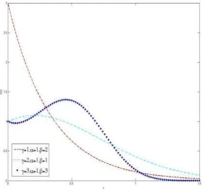
[image:3.595.65.276.550.749.2]where γ > 0, α, β ≥ 0 such that α +β > 0. It is clear that the MWD is very flexible. This is so since there are many other distributions that can be considered as special cases of MWD, by selecting the appropriate values of the parameters. These special cases include four distributions as shown in Table (I). In Figures (2-4) there are the distributions generated from MWD by changing the parameters.
Fig 2. The MWD with fixed α=1.
Fig3. The MWD with fixed γ =2.
Fig.4. The MWD with fixed β=1.
6.
PARAMETER
ESTIMATION
To estimate the parameters of MWD, the maximum likelihood is used. Let Let 𝐗𝟏, 𝐗𝟐… , 𝐗𝐧 be a sample of size N from an
MWD. Then the log-likelihood function (𝓛) is given by:
ℓ= 𝑛𝑖=1𝑓𝑖 𝑥 = 𝑛𝑖=1 ∝ +βγ𝑥𝑖𝛾−1 × exp −∝ 𝑥𝑖−
𝛽𝑥𝑖𝛾 (17)
Hence, the log likelihood function ℒ = lnℓbecomes
ℒ = logℓ= log ∝ +βγ𝑥𝑖𝛾−1 𝑛
𝑖=1
× exp −𝑥𝑖− 𝛽𝑥𝑖𝛾 18
ℒ = logℓ= 𝑛𝑖=1 log ∝ +βγ𝑥𝑖𝛾−1 × exp −∝ 𝑥𝑖−
Volume 179 – No.3, December 2017 ℒ = logℓ= log ∝ +βγ𝑥𝑖𝛾−1
𝑛
𝑖=1
+ log exp −∝ 𝑥𝑖− 𝛽𝑥𝑖𝛾 𝑛
𝑖=1
(20)
ℒ = logℓ= 𝑖=1𝑛 log ∝ +βγ𝑥𝑖𝛾−1 + 𝑛𝑖=1 −∝ 𝑥𝑖−
𝛽𝑥𝑖𝛾 21
Therefore, maximum likelihood estimation of α, β and γ are derived from the derivatives of ℒ.They should satisfy the following equations:
𝜕ℒ 𝜕𝛼= 0 ,
∂ℒ ∂β= 0 ,
∂ℒ ∂γ= 0 𝜕ℒ
𝜕𝛼 = 1 ∝ +βγ𝑥𝑖𝛾−1 𝑛
𝑖=1
− n𝑥𝑖 22
𝜕ℒ 𝜕𝛽 =
γ𝑥𝑖𝛾−1
∝ +βγ𝑥𝑖𝛾−1 𝑛
𝑖=1
− 𝑥𝑖𝛾 𝑛
𝑖=1
23
𝜕ℒ 𝜕𝛾=
β𝑥𝑖𝛾+1+ 𝛽γ𝑥𝑖𝛾 log 𝑥𝑖
∝ +βγ𝑥𝑖𝛾−1 𝑛
𝑖=1
− 𝛽𝑥𝑖𝛾 log 𝑥𝑖 𝑛
𝑖=1
24
To estimate the value of parameters, the system of equations (22-24) must be solved. However, it is difficult to solve this system so, the genetic algorithm (GA) [23-24] will be used as an alternative numerical method to estimate the parameters. The GA optimization technique lies in the fact that it can minimize the negative of the log-likelihood objective function in (11), essentially without depending on any derivative information.
7.
NUMERICAL
RESULTS
[image:4.595.55.282.74.324.2]Numerical experiments show that the GA method converges to an acceptably accurate solution with substantially fewer function evaluations. We have generated random number from MWD with parameters α, β and γ. By performing GA, we obtained the best estimation of parameters as in table (II).
Table 1: Parameter estimation by using GA
𝛼 𝛽 𝛾 𝛼 𝛽 𝛾 Err
X1 3 4 2 2.97 4.11 1.86 0.02
X2 5.2 6.8 2.5 5.27 6.80 2.42 0.06
X3 1.9 8.2 5.7 1.98 8.12 563 0.006
We resolve to FastICA algorithm for blind image separation. This algorithm depends on the estimated parameters and an un-mixing matrix W which estimated by FastICA algorithm. By substituting (22) into (19) for the source estimates ul,l =
1, 2, . . . , n, it becomes clear that the proposed score function inherits a generalized parametric structure, which can be attributed to the highly flexible MWD parent model. So, a simple calculus yields the flexible BSS score function
𝜑_𝑙 (𝑢_𝑙 ) = −𝑑/(𝑑𝑢_𝑙 ) log[( ∝ +βγ𝑥^(𝛾 − 1) ) × exp{ −∝ 𝑥 − 𝛽𝑥^𝛾 } ] (25)
In principle φl ul|θ is capable of modeling a large number of
signals as well as various other types of challenging heavy- and light-tailed distributions. Experiments were done to investigate
the performance of our method through three applications (two in source separation and one in image denoising) when impulsive noise is presented. In all experiments, the performance of our method is compared with generalized gamma [26], tanh, skew, pow3 [25], and Gauss [15]. Our performance is measured by the peak-signal-to- noise ratio (PSNR), defined as:
𝑷𝑺𝑵𝑹 = 𝟐𝟎 𝐥𝐨𝐠𝟏𝟎
𝟐𝟓𝟓
𝑴𝑺𝑬 𝟐𝟔
Table 2 Image separation PSNR
Distribut ion / PS NR First Im ag e Second Ima ge Thi rd Ima ge Forth Ima g e El apse d time (in sec onds)
MSE PSNR MSE PSNR MSE PSNR MSE PSNR
Skew 0.
1268 57.0987 0.1113 57.6649 18070. 55.5620 0.0851 58.8299 6.487527
Gauss 0. 0016 76. 0944 0. 0085 68. 8500 0. 0054 70. 7811 0. 1000 58. 1294 7. 636851 Ta nh 0.
0016 76.0275 0.0086 68.8042 0.0051 71.0909 5.0284e
-04 81. 1165 6. 211509 Gene ra lize d
Gamma 0.0053 70.9873 0.0055 70.7157 0.0074
69. 4270 9. 0603e -05 88. 5594 5. 690457 Pow 3 0.
2731 53.7671 0.0089 68.7042 00490. 71.1809 0.0991 58.1708 10.957964
Modifie d We ibu ll 0.
0042 71.8604 0.0053 70.8845 0.0080 69.0955 4.9152e
-05 91.
2154
5.
199108
[image:4.595.69.273.480.600.2]Volume 179 – No.3, December 2017
Fig. 5. Medical image denoising using Gauss filter: A, D are the source images, B, E are the noised images, C, F are the
[image:5.595.318.531.268.439.2]denoised images.
Fig. 6. Medical image denoising using Skew filter: G, J are the source images, H, K are the noised images, I, L are the
denoised images.
Fig7. Medical image denoising using Pow3 filter: M, P are the source images, N, Q are the noised images, O, R are the
[image:5.595.64.278.285.451.2]denoised images.
Fig. 8. Medical image denoising using Tanh filter: A, D are the source images, B, E are the noised images, C, F are the
denoised images.
Fig. 9. Medical image denoising using generalized gamma filter: G, J are the source images, H, K are the noised
images, I, L are the denoised images.
[image:5.595.62.281.459.657.2] [image:5.595.311.534.483.658.2]Volume 179 – No.3, December 2017
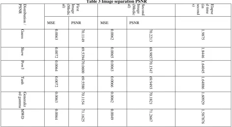
Table 3 Image separation PSNR
Distrib
u
tio
n
/
PSNR Im First
ag e (M ed ic al) Seco n d Im ag e (M ed ic al) Elaps e d tim e (in seco n d s)
MSE PSNR MSE PSNR
Gau ss 0 .00 6 3 7 0 .11 4 9 0 .00 6 2 7 0 .22 1 3 1 .98 7 5 Sk ew 0 .00 7 2 6 9 .53 9 4 0 .00 6 5 6 9 .98 5 7 1 .84 4 6 Po w3 0 .00 6 4 7 0 .06 0 0 0 .00 6 3 7 0 .15 4 7 1 .64 0 4 5
Tanh 0.00
7 2 6 9 .55 8 0 0 .00 6 6 6 9 .94 9 3 1 .64 8 8 6 Gen eraliz ed
gamma 0.00
6 3 7 0 .11 5 4 0 .00 6 2 7 0 .18 2 1 1 .60 9 2 9
MWD 0.00
6 4 7 1 .16 2 5 0 .00 4 9 7 1 .26 6 7 1 .58 7 8 7 6
8.
CONCLUSION
In this paper, we introduced a new technique for image denoise and blind image separation based on exponentiated transmuted Weibull distribution. Our proposed technique outperforms existing solutions in terms of separation quality and computational cost. Using the GA to estimate the parameters of MWD gives small error. Also, the results of MWD are better than other algorithms.
9.
REFERENCES
[1] Y. Zhang and Y. Zhao, 2013. Modulation domain blind speech separation in noisy environments, Speech Communication, vol. 55, no. 10, pp. 1081–1099.
[2] M. T. ¨ Ozgen, E. E. Kuruoˇglu, and D. Herranz, 2009. Astrophysical image separation by blind time-frequency source separation methods, Digital Signal Processing, vol. 19, no. 2, pp. 360–369.
[3] Ikhlef, K. Abed-Meraim, and D. Le Guennec, 2010. Blind signal separation and equalization with controlled delay for MIMO convolutive systems, Signal Processing, vol. 90, no. 9, pp. 2655– 2666.
[4] R. Romo V´azquez, H. V´elez-P´erez, R. Ranta, V. Louis Dorr, D. Maquin, and L. Maillard, Blind source separation, 2012. Wavelet denoising and discriminant analysis for EEG artifacts and noise cancelling, Biomedical Signal Processing and Control, vol. 7, no. 4, pp. 389–400.
[5] M. Babaie-Zadeh and C. Jutten, 2005. A general approach formutual information minimization and its application to blind source separation, Signal Processing, vol. 85, no. 5, pp. 975–995.
[6] K. Todros and J. Tabrikian, 2007. Blind separation of independent sources using Gaussian mixture model, IEEE Transactions on Signal Processing, vol. 55, no. 7, pp. 3645–3658.
[7] E. Oja and M. Plumbley, April 2003. Blind separation of positive sources using nonnegative PCA, in Proceedings of the 4th International Symposium on Independent Component Analysis and Blind Signal Separation (ICA ’03), Nara, Japan, pp. 11–16.
[8] M. Kuraya, A. Uchida, S. Yoshimori, and K. Umeno, 2008. Blind source separation of chaotic laser signals by independent component analysis, Optics Express, vol. 16, no. 2, pp. 725–730.
[9] P. Comon, 2014. Tensors: a brief introduction, IEEE Signal Processing Magazine, vol. 31, no. 2, pp. 44–53.
[10]W. L. Woo and S. S. Dlay, 2005. Neural network approach to blind signal separation of mono-nonlinearly mixed sources, IEEE Transactions on Circuits and Systems I, vol. 52, no. 6, pp. 1236–1247.
[11]Cichocki and R. Unbehauen, 1996. Robust neural networks with on-line learning for blind identification and blind separation of sources, IEEE Transactions on Circuits and Systems I: Fundamental Theory and Applications, vol. 43, no. 11, pp. 894–906.
[12]S.-I. Amari, T.-P. Chen, and A. Cichocki, 1997. Stability analysis of learning algorithms for blind source separation, Neural Networks, vol. 10, no. 8, pp. 1345–1351.
[13]K. Kokkinakis and A. K. Nandi, 2005. Exponent parameter estimation for generalized Gaussian probability density functions with application to speech modeling, Signal Processing, vol. 85, no. 9, pp. 1852–1858.
Volume 179 – No.3, December 2017 [15]E. W. Stacy, 1962. A generalization of the gamma
distribution, Annals of Mathematical Statistics, vol. 33, no. 3, pp. 1187–1192.
[16]Sarmiento, I. Durán-Díaz, A. Cichocki, and S. Cruces, 2015. A contrast based on generalized divergences for solving the permutation problem of convolved speech mixtures, IEEE/ACM Transactions on Audio, Speech, and Language Processing, Vol. 23, no. 11, pp. 1713-1726.
[17]J. Eriksson, J. Karvanen, and V. Koivunen, 2002. Blind separation methods based on Pearson system and its extensions, Signal Processing, vol. 82, no. 4, pp. 663–673.
[18]J. Karvanen, J. Eriksson, and V. Koivunen, 2002. Adaptive Score Functions for Maximum Likelihood ICA, The Journal of VLSI Signal Processing, Vol. 32, no 1-2, PP 83-92.
[19]J. Karvanen, J. Eriksson, and V. Koivunen, June 2000. Source distribution adaptive maximum likelihood estimation of ICA model, in Proceedings of the 2nd International Conference on ICA and BSS, Helsinki, Finland, pp. 227– 232.
[20]Aapo Hyvärinen and Erkki Oja, 2000, Independent Component Analysis: Algorithms and Applications, Neural Networks, vol.13, no. (4-5), pp. 411-430
[21]C. Jutten and J. Karhunen, 2004, “Advances in blind source separation (bss) and independent component analysis (ica) for nonlinear mixtures.”, Int J Neural Syst, vol. 14, no. 5, pp. 267–292.
[22]Mazen Zaindin, Ammar M. Sarhan, 2009, Parameters Estimation of the Modified Weibull Distribution, Applied Mathematical Sciences, Vol. 3, no. 11, pp. 541 – 550.
[23]M. Li and J. Mao, June 2004. A new algorithm of evolutional blind source separation based on genetic algorithm, in Proceedings of the 5th World Congress on Intelligent Control and Automation, Hangzhou, Zhejiang, China, pp. 2240–2244.
[24]S. Mavaddaty and A. Ebrahimzadeh, December 2009. Evaluation of performance of genetic algorithm for speech signals separation, in Proceedings of the International Conference on Advances in Computing, Control and Telecommunication Technologies (ACT’09), Trivandrum, Kerala, India, pp. 681–683.
[25]A. Hyvarinen, J. Karhunen, and E. Oja, 2001. Independent Component Analsysis, JohnWiley & Sons.
[26]Internet web: http://sipi.usc.edu/database/database.cgi