RESEARCH ARTICLE
DETERMINANTS OF COST EFFICIENCY AMONG SUGARCANE FARMERS: A STOCHASTIC
FRONTIER COST FUNCTION APPROACH
*Dr. Rangalal Mohapatra
Department of Economic Studies and Planning, Sikkim University, 6
thMile, Samdur,
Po- Tadong, Gangtok, Sikkim-737102
ARTICLE INFO ABSTRACT
The stochastic Frontier cost model was used to analyze the cost efficiency of Sugarcane farm households of Odisha. The primary data were collected from the 200 sugarcane farm households. The joint estimation of parameters of cost function and inefficiency model through one step maximum likelihood method showed that the 97% of the inefficiency were explained due to cost inefficiency and cost efficiency could be increased by 36% through better use of available farm resources. Since college education, average education of the family and experience significantly reduced cost efficiency, this could be achieved through farm specific inputs which include improved education of the effective farm household, better experience, improved education of the family and participation of more educated youth in farming practices. In addition to this, policy should be made for encouraging farm practices in higher education system so that formal education system can link agricultural system of the economy.
Copyright, IJCR, 2013, Academic Journals. All rights reserved.
INTRODUCTION
Agriculture is a way of life, which for centuries has shaped the thought, the outlook, the culture and the economic life of the people of India. Despite a steady decline of the share of agriculture in national income, the overall growth rate of the economy is largely determined by the performance of the agricultural sector. The pioneering work of Schultz, (1964), made it clear to many that to improve the lot of the poor people in low-income developing countries are not “space, energy and crop land; the determining factor is improvement in the human quality” Schultz (1971). Schultz (1981) in his ‘investing in the human capital’ pointed out that one of the fundamental mistakes done by the economists is understanding the human agents in agriculture–farm laborers and farm entrepreneurs who both work and allocate resources in the production. In the process of transforming agriculture from a traditional to a modern, dynamic and progressing state (from mid-Sixties onwards), not only the primary inputs but other non-tangible factors such as levels of schooling experience that brings a change in the quality of the human agent in using the available technology under the broad category of ‘human capital’ also play a vital role in improving production and productivity in farm production.
The complementarities of education with the access to new information, decoding the relevant information, the use of new inputs, adoption of new methods of production and reaping the maximum benefit out of it makes it very much useful to make an attempt to study the various forms of human capital such as formal schooling in various forms in addition to other primary inputs on improving individual farm efficiency. The productive value of education has its root in two distinct phenomena such as worker effect and allocative effect. Increased education simply may permit a worker to accomplish more with resources at hand. This ‘Worker effect’ is the marginal product of education as it is normally defined,
*Corresponding author: [email protected],
that is the increased output per unit change in education holding other factor quantities constant. On the other hand, increased education may enhance the worker’s ability to acquire and decode information and cost and productive characteristics of other inputs. As such a change in education results in a change in other inputs including perhaps the use of some new factors that otherwise would not have used. This is called allocative effect. In a pioneering study exploring
the economic effects of education, Grilliches (1958)used production
function analysis to highlight the contribution of education in agricultural productivity. However, following Welch (1970), the subsequent literature has not deemed it necessary to maintain the distinction between the innovative and allocative effect. Evidence from 13 low-income countries shows that farm productivity, on an average, increases by 8.7 percent as a result of a farm completing
four years of elementary education (Lockheed et al., 1980).
Bikhauser et al. (1991) reviewed Forty-seven studies from 17
countries and found that 33 studies show significant and positive extension effect. Research towards identifying and understanding the role of education in production can be categorized into two parts.
In the first part, the technical efficiency part is investigated between two groups of farmers either educated or uneducated or traditional
and modern farmers (Welch, 1970; Moock, 1981; Lockheed et al.,
1980; Pudasaini, 1983; Azhar, 1991). The studies analyzed both
technical and allocative effect part of education are (Welch, 1970; Ram, 1980; Pudasaini, 1982, 1983; Duraiswamy, 1990, 1992; Mohapatra, 1998). A detailed review is presented in Tilak (1993). The pioneering work of Farrell (1957) on the measurement of efficiency and the introduction of stochastic frontier models,
independently proposed by Aigner, Lovelland Schmidt (1977) and
Meeusen and Vanden Broeck (1977) and extended by Jondrow et al.,
(1982) brought a large number of empirical studies of measuring technical, allocative and economic efficiency of the farms with special reference to education age and experience of the farms using cross sectional data (Kalirajan 1981, 1990; Sqires and Tabor 1991; Bravo-Ureta and Pinheiro,1997; Hwang and Bagi 1984; Ogundari
et al., 2006). According to the studies reviewed by Bravo-Ureta and
Pinheiro (1993), it can be argued with justification that stochastic
ISSN: 0975-833X
International Journal of Current Research
Vol. 5, Issue, 03, pp. 634-638, March,2013
INTERNATIONAL JOURNAL
OF CURRENT RESEARCH
Article History:
Received 07th December, 2012 Received in revised form 09th
January, 2013
Accepted 04th February, 2013 Published online 19th March, 2013
Key words:
Effective head of the Household, Cost Efficiency,
models are more reliablethan the deterministic models because the former account for statistical noise In case of the simple Cobb-Douglas production function, on an average, the percentage gain in output for each year of education is around 3.5 %. In case of the stochastic frontier methodology using the cross section data, the TE and AE are 70% and 68%. The average TE and EE for the studies using dual frontier are 88% and 69% respectively and TE, AE and EE for the studies using deterministic frontier are 63%, 68% and 32 % respectively. This paper aimed at better understanding of small scale sugarcane farmers of the study area (Jajpur district of Odisha) with a view to predicting cost efficiency (a measure of farm’s ability to produce at a given level of output using cost minimization input ratio of 200 farmers), using stochastic frontier cost function in which the maximum likelihood estimates of the parameters of cost function and the linear inefficiency function have been obtained jointly through FRONTIER-4.1c Coelli (1996). The differences in cost efficiency among the farm households are explained with special reference to schooling of the farmers, education of the family and experience of the farm household.
MATERIALS AND METHODS
The data used in this paper are directly collected from the farm households of the study area (Goleipur Panchayat of Korei block, Jajpur district, Odisha) through a questionnaire. The specific area of the study is chosen because of its well road and transport connectivity through National Highway, multi-cropping pattern and existence of big markets. With a formal permission taken from the sarapancha of the Village Panchayat, Six villages have been selected for collecting information from 200 farm households. The stochastic frontier approach, based on specific functional form introduced by Aigner, Lovell Schmidt (1977) and Meeusen and Van den Broeck (1977), is motivated by the idea that the deviation from the frontier may not be entirely attributed to the inefficiency because random shocks outside the control of the farmers can also affect the output. The cost function can be used simultaneously to predict both technical and allocative efficiency of a farm (Coelli, 1995). Also it can be used to resurrect all the economically relevant information about farm level technology as it is generally positive, non-decreasing, concave continuous and homogeneous to degree one to input prices (Chambers, 1983). In this
study, Battesse and Coelli (1995) model is used to specify a
stochastic frontier cost function with behavior inefficiency component and to estimate all parameters together in one step maximum likelihood estimation. The model is implicitly expressed as:
Ln Ci = g(Yi, Pi: α) + (νi+υi ) ---1
Where Ci represents the total cost of production of the ith farm
household; g is a suitable functional form such as Cobb-Douglas;
Pi is a vector variable of input prices: Yi is sugarcane output in Kgs;
α is the parameter to be estimated. The systematic component
νi represents random disturbances of cost due to factors outside the
scope of the farmers. It is assumed to be identically and normally
distributed with mean zero and constant variance as N (0, σν 2) . υi is
the one sided disturbance form used to represent cost inefficiency and
is independent of νi . Thus υi =0 for a farm whose cost lie on the
frontier, υi > 0 whose cost lie above the frontier; υi < 0 whose cost lie
below the frontier. υi is identically and independently distributed as
N(0, συ 2). The two error terms are proceeded by positive signs
because inefficiencies are always assumed to increase the cost. Cost
efficiency1 (CEE) of an individual farm is defined in terms of the ratio
of observed cost (COB) to the corresponding minimum cost (CMIN)
given the available technology.
1
In this cost function Ui now defines how far the farm operates above the cost frontier. If
allocative efficiency is assumed, the ui is closely related to the cost of technical
inefficiency. If this assumption is not made, the interpretation of ui in a cost function is
less clear, with both technical and allocative inefficiencies involved. Thus we shall refer to efficiencies measured relative to a cost frontier as ‘cost’ efficiencies in this document. The exact interpretation of these cost efficiencies will depend upon the particular application.
(CEE ) = (COB)/ (CMIN ) = {g(Yi, Pi: α) + (νi+υi ) / g(Yi, Pi: α) + (νi)}=
exp(νi ) ---(2)
(CEE) takes 1 or higher than 1 defining cost efficient farm. Following
the adoption of Battesse and Coelli (1995) framework for the analysis of data, the explicit Cobb-Douglas functional form for the sugarcane data of the study area is, therefore, specified as:
Ln Csi = ln αo+ α1 ln Y1i + α2 ln P1i + α3 ln P2i + α4 ln P3i+ α5 ln P4i +
α6 ln P5i +α7 ln P6i + (νi+υi ) ---(3)
Itrepresents the Frontier total cost function for sugarcane production
of the study area; Cpi stands for the total cost (in Rs.) of production
for the ith farm; Yi stands for the total sugarcane output (in Kg.)
produced by the ith farm household. In equation (3), P1 to P6
represent cost of labor, cbullock labor, Nitrogen, irrigation and cost of tractor hours The choice of the Cobb-Douglas functional form is based on the fact that the function is self-dual as in the case of cost function in which the present analysis is based on. The inefficiency models for the above sugarcane cost frontier is defined as:
Usi= δo + δ1EF + δ2EX+ δ3 E + D1EDU +D2EDU +D3EDU ---(4)
Where, Usi are the cost inefficiency component for sugarcane. EF
refers to the average education of the family; EX represents the experience of the effective head of the household; E refers to the levels of formal schooling year completed by the effective head farm
household2 and D1 refers to education dummy for college level
education; D2 represents the higher secondary education dummy and
D3 represents the primary and higher primary schooling dummy.
These exogenous intangible variables are included to examine their
impact on the cost efficiency of the farmers. The δi s and Di s are the
scalar parameters to be estimated. The variance of the random error,
σν 2 , and the cost inefficiency error συ 2 and overall variance of the
model σ2 are related as follows: γ = συ 2 / (σν 2 + συ 2 ). The Gamma
(γ) measures the total variation of the total cost from the frontier cost
which can be attributed to cost inefficiency (Battesse and Corra, 1977). The estimates for all the parameters are simultaneously obtained using the programme FRONTIER 4.1 (Coelli, 1996). The test for the presence of cost inefficiency using generalized likelihood
ratio statistics λ obtained by λ = -2ln (Ho/Ha). If the null hypothesis is
true then λ has approximately a mixed chi-square distribution with
degrees of freedom equal to the number of parameters excluded in the unrestricted model.
RESULTS AND DISCUSSION
Table 1 is presented with the summary statistics of the variables in the sugarcane stochastic cost frontier model. The mean total cost of
sugarcane cultivation is ₹ 11630 with minimum of ₹ 5554 and
maximum of ₹ 32075. The huge range of total cost clearly indicates
that the range of cultivation of sugarcane is also very high. Since more financial investment and more time are required, some farmers do not cultivate more area under the crop. The high labor cost share in the total cost is due to the fact that sugarcane cultivation takes longer period (18 months to 20 months), plenty of manual labor works are to be used; the use of labor power is comparatively more. Second thing is that, sugarcane cultivation requires use of different fertilizer in different times. Hence, the share of each fertilizer is estimated. The maximum share is by Nitrogen (Urea) is 4.74 per cent followed by calcium (3.01%) and Super (2.05%). The high share of irrigation cost (10.28%) also indicates the importance of continuous requirement of water in the sugarcane production. It should be
2 While collecting the sample, it has been observed that the head of the farm
household, most often, is not the real cultivator. Hence, the family member who cultivates the farm takes the major decision regarding farm production. Hence, he is designated by the term “effective head of the household”.
mentioned that most the farm households in the study area use diesel water pump (Five Horse Power) for irrigating their sugarcane fields. The significant share of the tractor hour is proved from the fact that, the traditional bullock driven plough wood cultivation cannot achieve deeper cultivation of the land, as it is essential for sugarcane crop. Secondly, the easy availability of tractors power tillers in the local area and the consequent hiring cost benefit for the farmers are another factor for the large share of the tractor cost in the total cost. The results of the joint estimation of the parameters of the stochastic Cobb-Douglas cost frontier for sugarcane are presented in the Table 2.
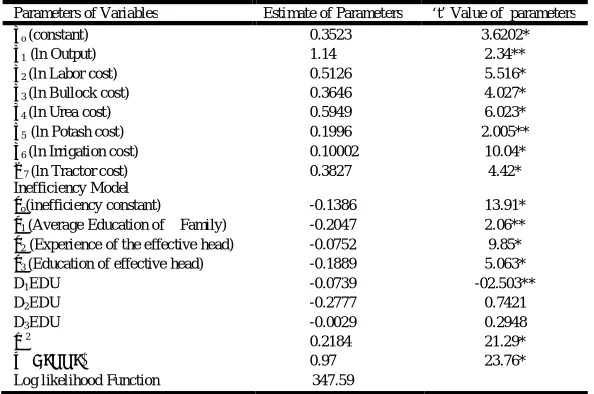
All the beta coefficients of the sugarcane stochastic frontier cost function were statistically significant. It shown the relevance of the input prices and the volume of output in the sugarcane cost function
of the study area. Sugarcane crop belongs to Gramineae, the grass
family. It responds well to nutrition and water management. Sugarcane productivity can increase if appropriate irrigation and fertilizer management is followed. Preparatory tillage is very important operation in sugarcane cultivation. Sugarcane roots penetrate up to 90 centimeters deep in the soil and, hence, for better growth tillage has an important effect. Soil preparation must destroy the stumps of the old canes and improve any bad physical soil characteristics or loss of structure those have developed during the previous year. In this background it can be argued that the importance of both bullock driven plough wood tilling and tractor tilling is very much prominent. The use of fertilizer such as nitrogen, potash and
phosphorous and irrigation is utmost essential. This in fact was revealed from the results of the statistically significant beta coefficients of the sugarcane frontier cost function of the study area. The model without inefficiency components was tested against the model with efficiency components and the null hypothesis that there is no difference between these two models was rejected at 1% level of significance. The likelihood function value for without inefficiency component was 101.78 and the corresponding value for
the alternative is 347.59. From the gamma value (γ), it was concluded
that 97% of the inefficiency was due to the cost inefficiency which was attributed to education of the family of the effective head of the household, experience of the effective head of the household and the education of the effective head.
All these factors, of course, contributed positively in reducing cost inefficiency, the differences came when the education of the effective head was used as a dummy variable. In case of college education, the
dummy D1 was statistically significant in reducing the cost
inefficiency in the sugarcane production. This supports the study
(Nandolnyak et al., 2006; Asogwa, 2011). Since sugarcane
production takes 16 to 18 months, lots of care has to be taken by the farmers. For example, preparation of the soil suited for plantation; preparation of plant cuttings and culture of plant cuttings, use of proper dose of fertilizer in appropriate time; choice of irrigation method such as, flood irrigation and drip irrigation. It was also realized that the farmers with more schooling specially college level are more prone to better management with efficient method of production as stated above, many farmers used drip irrigation which
Table 1. Summary Statistics of Variables in the Sugarcane Stochastic Cost Frontier Model (In Rupees)
Variable Mean (Rupees) Standard Deviation (Rupees)
Minimum (Rupees)
Maximum (Rupees)
% of the total cost
TC 11630 5554 5600 32075
VO 2709.5 1377.6 7080 51200
Labor cost 4576.8 2202 640 12400 39.35
Bullock labor cost 245.2 1335.7 840 10500 2.2
Urea cost 551.70 315.7 175 3750 4.74
Potash cost 230 149 80 1500 1.28
Super cost 239.55 126.87 60 750 2.05
Calcium cost 350.475 202.33 75 1125 3.01
Manure cost 34.31 18.47 12 120 0.3
Tractor cost 1906.5 983.85 600 5400 16.4
Irrigation cost 1195.6 598.04 160 4000 10.28
Average Education of the Family* 8.270 2.514 4 10
Average Education of the effective head* 8.13 2.35 3 13
Experience* 8.21 2.521 3 13
[image:3.612.159.456.248.445.2]*The figures are in number of years of farming experience in growing sugarcane
Table 2. Maximum-likelihood Estimates of Parameters of Cobb-Douglas Frontier Cost Function for the Sugarcane Farm Household
Parameters of Variables Estimate of Parameters ‘t’ Value of parameters
βo (constant) 0.3523 3.6202*
β1 (ln Output) 1.14 2.34**
β2 (ln Labor cost) 0.5126 5.516*
β3 (ln Bullock cost) 0.3646 4.027*
β4 (ln Urea cost) 0.5949 6.023*
β5 (ln Potash cost) 0.1996 2.005**
β6 (ln Irrigation cost) 0.10002 10.04*
Β7 (ln Tractor cost) 0.3827 4.42*
Inefficiency Model
δo(inefficiency constant) -0.1386 13.91*
δ1 (Average Education of Family) -0.2047 2.06**
δ2 (Experience of the effective head) -0.0752 9.85*
δ3 (Education of effective head) -0.1889 5.063*
D1EDU -0.0739 -02.503**
D2EDU -0.2777 0.7421
D3EDU -0.0029 0.2948
σ 2
0.2184 21.29*
γ (Gamma) 0.97 23.76*
Log likelihood Function 347.59
saved 30 to 40 per cent of the water and also thereby the diesel and electricity consumption also reduced accordingly. On the other side, the farmers with little education, of course, have contribution but not statistically significant. Some time the wrong choice of using bullock labor instead of tractor for initial cultivation reduces cost efficiency.
Ever since Chaudhuri (1974) has articulated this idea as “Lapses back
into illiteracy”. According to Nelson-Phelps-Schultz hypothesis
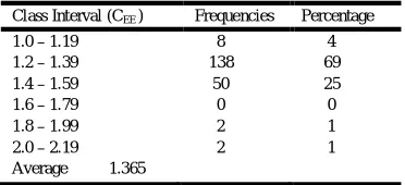
(1986) the effect of education is supposed to differ over time, as time passes and new technological diffusions are made in the field of agriculture, the knowledge from either primary schooling or from higher primary schooling will be totally useless in acquiring useful information and decoding them for the farm practices. Hence, the hypothesis that education of the effective farm households has positive and statistically significant impact is accepted. The frequency distribution table of farm level cost inefficiency, the corresponding frequency and its percentage of farm household belong to each category are presented in the Table 3. The frequency distribution of sugarcane cost efficiency scores are presented in the Table 3. The average efficiency score was 1.365. Sixty Nine per cent of the total farm households had scores in between 1.2 to 1.39 and 25 % were in the range of 1.4 to 1.59. There is chance that the cost inefficiency scores can be reduced, on an average, by 36 % in comparison to the frontier cost
Conclusion
The implication of the study is that the farmers were not minimizing the production cost indicating that the cost efficiency among the sugarcane farmers could be increased by 36 % through better use of the available resources given the current state of technology. This could be achieved through improved education of the farmer, improved farm experience, higher family education. The government should provide better incentives to the educated youths to actively participate in various farm management activities. More farm extension services to the farm households can improve the experience in practicing modern farm management practices thereby improving farm production and productivity helping an accelerated economic growth
REFERENCES
Aigner, D. J., Lovell, C. A. K and Schmidt, P. J. 1977. Formulation
and Estimation of Stochastic Frontier Production Model.
Journal of Econometrics., 6: 21-37.
Asogwa, B.C., Ihemeje, J.C. and Ezihe, J.A.C. 2011. Technical and Allocative Efficiency Analysis of Nigeria Rural Farmers
Implication: for Poverty Reduction. Agricultural Journal., 6(5):
243-251.
Azhar, R. A. 1991. Educational Efficiency During the Green
Revolution in Pakistan. Economic Development and Cultural
Change., 39 (3): 651-65 .
Battesse, G. E. and Coelli, T. J. 1995. A Model for Technical Inefficiency Effects in Stochastic Frontier Production for Panel
Data, Empirical Economics., 20: 325-45.
Battese, G. E., and Corra, G. S. 1977. Estimation of Production Frontier Model: With Application to the Pastoral Zone of
Australia. Australian Journal of Agricultural Economics., 21:
1969-79.
Birkhaeuser, D: Evenson, R.E. and Feder, G. 1991. The Economic Impact of Agricultural Extension: A Review, Economic Development and Cultural Change., 39 (3) : 607-50.
Bravo-Ureta, B. E., and Pinheiro, E. A. 1997. Technical, Economic and Allocative Efficiency in Peasant Farming: Evidence from
Dominican Republic, The Developing Economics., XXXV(1):
48-67.
Bravo-Ureta, B. E., and Pinheiro, E. A. 1993. Efficiency Analysis of Developing Country Agriculture: A Review of the Frontier
Function Literature. Agricultural and Resource Economics
Review, 22(1): 88-101.
Chambers, R. G. 1983. Applied Production Analysis: A Dual Approach, Cambridge: Cambridge University Press.
Choudhuri, D. P. 1974. Effect of Farmer Education on Agricultural Productivity and Employment: A Case Study of Punjab and
Haryana States of India (1960-72), Mimeographed, Armidale:
University of New England.
Coelli, T.J. 1995. Recent Developments in Frontier Modeling and
Efficiency Measurement. Australian Journal of Agricultural
Economics., 39: 219-245.
Coelli, T.J. 1996. A Guide to FRONTIER Version 4.1c: A Computer Programme for Stochastic Frontier Production and Cost Function Estimation, Working Paper 96/07, Centre for Efficiency and Productivity Analysis, Dept. of Econometrics, University of New England, Armidale, Australia.
Duraiswamy, P. 1992. Effects of Education and Extension Contact.
Indian Journal of Agricultural Economics., 47( 2): 205-14.
Duraiswamy, P. 1990, Technical and Allocative Efficiency of Education in Agricultural Production: A Profit Function Approach, Indian Economic Review., 25(1):17-32.
Farrell, M. J. 1957. The Measurement of Productive Efficiency.
Journal of Royal Statistical Society, A120( 3): 253-281.
Grilliches, Z. 1958. Research Costs and Social Returns: Hybrid Corn
and Related Innovations, Journal of Political Economy, 66(5):
419-431.
Huang, C. J. and Bagi, F. S. 1984. Technical Efficiency on
Individual Farms in Northwest India. Southern Economic
Journal., 51: 108-15.
Jondrow, J, Knot C. A, Materov, L V and Schmidt Peter, 1982. On the Estimation of Technical Efficiency in the Stochastic Frontier
Production Function Model. Journal of Econometrics., 19, (2/3):
233.38.
Kalirajan, K. 1981. The Economic Efficiency of Farmers Growing
High Yielding Irrigated Rice in India. American Journal of
Agricultural Economics., 63, (3): 566-70.
Kalirajan, K. 1990. On Measuring Economic Efficiency. Journal of
Applied Econometrics., 5: 75-85.
Lockheed J., Jamison, D. T. and Lau, L.J. 1980. Farmer Education
and Farm Efficiency: A Survey. Economic Development and
Cultural Change., 29(1): 37-76.
Meeusen, W. and Broec, V. D. 1977. Efficiency Estimation from Cobb-Douglas Production Function with Composed Error.
International Economic Review., 18: 435-445.
Moock, P. R. 1981. Education and Technical Efficiency in Small
Farm Production. Economic Development and Cultural
Change., 29: 722-39.
Mohapatra, R. 1998. Effects of Education on Technical and Allocative Efficiency in Farm Production: Evidence from
Orissa. The Indian Journal of Economics., 79( 312): 81-98.
Nadolnyak, D. A., Fletcher, S. M. and Hartarska, V.M. 2006. Southeastern Pea-nut Production Cost Efficiency Under the Quota System: Implication for the Farm Level Impact of 2002.
Farm Journal of Agricultural and Applied Economics., 38(1):
213-251.
Nelson, R and Phelps, E. 1966. Investment in Humans Technological
Diffusion and Economic Growth. American Economic Review.,
56: 69-75.
[image:4.612.86.272.303.388.2]Ogundari, K. and Ojo, S.O. 2006. An Examination of Technical, Economic and Allocative Efficiency of Small Farms: The Case
Table 3. Frequency Distribution of Cost Efficiency for Sugarcane Farm-households
Class Interval (CEE ) Frequencies Percentage
1.0 – 1.19 8 4
1.2 – 1.39 138 69
1.4 – 1.59 50 25
1.6 – 1.79 0 0
1.8 – 1.99 2 1
2.0 – 2.19 2 1
Average 1.365
Study of Cassava Farmers in Osun State of Nigeria. Journal of
Central European Agriculture., 7(3): 423-42.
Ogundary, K. 2006. Determinants of Profit Efficiency Among Small Scale Rice Farmers in Nigeria: A Profit Function Approach, Paper Presented at International Association of Agricultural Economist Conference, Australia, August: 12-18
Pudasaini, S. 1983. The Effects of Agriculture: Evidence from Nepal.
American Journal of Agricultural Economics., 65: 509-515.
Pudasaini, S. 1982. The Contribution of Education to Allocative Efficiency in Sugarcane Production in Nepal, Washington DC: The World Bank Population and Human Resource Division, Disc. Paper, 82: 8-55.
Ram, R., 1980. Role of Education in Production: A Slightly New
Approach. Quarterly Journal of Economics., 95(September):
365-73.
Schultz, T. W. 1964. Transforming Traditional Agriculture, New
Haven, and City: Yale University Press.
Schultz, T. W. 1971. Investment in Human Capital, Free Press, New York.
Schultz, T. W. 1981. Investing in People, University of California Press, Berkeley, USA.
Squires, D. and Tabor, S. 1991. Technical Efficiency and Future
Production Gain in Indonesian Agriculture. The Developing
Economies, 29: 258-70.
Tilak, J. B.G. 1993. Education and Agricultural Productivity in Asia:
A Review. Indian Journal of Agricultural Economics.,
48(2):187-200.
Welch, F. 1970. Education in Production. Journal of Political
Economy, 78(1): 35-59