Warm quintessential inflation

arXiv:1906.09648v3 [gr-qc] 9 Jul 2019

Warm Quintessential Inflation

Konstantinos Dimopoulos

_{and Leonora Donaldson-Wood}

Consortium for Fundamental Physics Physics Department, Lancaster University

Lancaster, LA1 4YB, UK

Abstract

We introduce warm quintessential inflation and study it in the weak dissipa-tive regime. We consider the original quintessential inflation model, which approxi-mates quartic chaotic inflation at early times and thawing quartic inverse-power-law quintessence at present. We find that the model successfully accounts for both infla-tion and dark energy observainfla-tions, while it naturally reheats the Universe, thereby overcoming a major problem of quintessential inflation model-building.

1

Introduction

Inflation is overwhelmingly the best mechanism for explaining the observed structure in the Universe as well as its spatial flatness and large-scale homogeneity [1]. In the same time, the discovery of dark energy [2] is best attributed to a non-zero, albeit incredibly fine-tuned, cosmological constant in the benchmark paradigm of ΛCDM [3]. However, recently both proposals have been challenged by the swampland conjectures [4], which stipulate the impossibility of de-Sitter vacua in string theory and also set stringent constraints on inflation model-building and undermine ΛCDM [5] (but see also Ref. [6]). Such constraints are not possible to meet with conventional inflation [7]. A successful way to model inflation while satisfying the swampland conjectures is incorporating dissipating effects [8], as in warm inflation [9]. On the dark energy front, the observations of the current accelerated expansion can be explained by quintessence instead of a non-zero cosmological constant Λ [10], which is also in agreement with the swampland conjectures [11]. In this letter, we attempt to join the two and introduce warm quintessential inflation (for a reference list on quintessential inflation see Refs. [12, 13]), which has the additional advantage of providing a natural mechanism for reheating the Universe. Reheating is of particular significance in quintessential inflation because the conventional reheating by the decay of the inflaton field at the end of inflation cannot occur as the field needs to survive until the present and become quintessence. We use natural units where c= ¯h =kB= 1 and 8πG =m−P2, where

mP = 2.43×1018GeV is the reduced Planck mass.

1

[email protected]

2

2

The model

The original quintessential inflation model is [14]3

V(φ) =

 



λ(φ4_+M4_{) for φ <0}

λM8

φ4_+M4 for φ >0

, (1)

where 0< M _≪ mP. For negative values of the inflaton fieldφ ≪ −M, the above potential

reduces to quartic chaotic inflation, which has been excluded by observations unless it is “warmed up”, by considering significant dissipation effects. During inflation φ ∼ −mP.

For positive values of the field φ_≫ M the potential becomes inverse power-law (IPL) quintessence. Such quintessence models feature a tracker solution, which however, is too steep to satisfy observations in the case of an inverse quartic potential V ∝φ−4_{. However,} in our case, the field does not follow the tracker but, after the end of inflation, it rushes down its runaway potential and freezes at a value φF ∼mP with some residual potential

density, which explains dark energy. At present, the field unfreezes and begins slowly rolling down its potential. Such quintessence is called “thawing” [16].

While the field runs from inflation at φ _{∼ −}mP to quintessence at φ∼mP it is

ki-netically dominated and oblivious of the potential [17]. Thus, the awkward discontinuity (in the fourth derivative) of the potential in Eq. (1) is not felt. In fact, the potential in Eq. (1) is only experienced by the field when _|φ_{| ∼}mP, which means that Eq. (1) is only

a guideline to the actual form of V(φ) and should not be taken too seriously.

In addition, the field runs over super-Planckian distance from the end of inflation to its eventual freezing. It is likely that the dissipative properties of the field are different in these two different patches of the scalar potential, which are several Planck scales apart. Indeed, we assume that dissipative effects are important only when the field is slow-rolling during inflation withφ_{∼ −}mP. Additionally, we consider only the weak dissipative regime, where

the dynamics of the field are not affected by dissipation (no extra friction) so this issue is not of our concern.

In the weak dissipative regime, the only effect of dissipation is that the quantum fluctu-ations of the inflaton field during inflation are superseded by its thermal fluctufluctu-ations, due to a subdominant thermal bath, generated and maintained by the dissipative effects. At the end of inflation, this thermal bath suffices to reheat the Universe, thereby overcoming one of the major problems of quintessential inflation model-building. Indeed, reheating cannot be due to inflaton decay, as in conventional inflation, because the inflaton must survive until today. A number of reheating mechanisms have been put forward, the most important of which are gravitational reheating [18], instant preheating [19], curvaton re-heating [20] and recently non-minimal rere-heating [21] (also called Ricci rere-heating [22]). In most cases, an extra degree of freedom must be assumed, which is coupled to the inflaton (instant reheating) or not (curvaton or non-minimal reheating), the only exception being gravitational reheating, which however is in danger of producing excessive tensors [23]. In this paper, efficient reheating occurs naturally without any additional assumptions.

3

3

Warm inflation

The slow-roll equations in warm inflation are

3H(1 +Q) ˙φ _{≃ −}V′ ₍₂₎

and ρr ≃

3 4Qφ˙

2_{, (3)}

where H is the Hubble scale, ρr is the density of the subdominant radiation, Q≡Υ/3H

with Υ being the dissipation coefficient and the dot (prime) denotes differentiation with respect to time (the inflaton field). The scalar power spectrum in warm inflation is [24]

Pζ =

H2_{(1 +Q)}2_F 8π2_εm2

P

, (4)

where ε is the inflationary slow-roll parameter (defined later, in Eq. (8)) and

F ≡1 + 2_N∗+ T

H

2πQ

q

1 + 4₃πQ, (5)

with _N∗ = (eH/T ₋₁₎−1 _{being the statistical distribution of the inflaton field at horizon} crossing, and T is the temperature of the subdominant thermal bath during inflation.4 In cold inflation, Q, T = 0 and F = 1 so that Eq. (4) reduces to the usual expression. However, in warm inflationT _≫H and so_{N∗ ≃}T /H _≫1. As mentioned, we consider the weak dissipative regime, where Q <1. In this case, Eq. (5) suggests _{F ≃}2(1 +πQ)T /H. For the density of the subdominant thermal bath we have

ρr =

π2 30g∗T

4 ₌ εQV

2(1 +Q)2 , (6)

whereg_∗ is the effective relativistic degrees of freedom and we used the slow-roll Friedman equation V _≃3m2

PH2 and Eqs. (2) and (3) in the last equation. Combining Eqs. (4) and

(6) we arrive at

Pζ =

1 4π2

45

π2_g ∗

!1/4

Q1/4_{(1 +Q)}3/2_{(1 +πQ)}

ε3/4

H

mP 3/2

. (7)

Now, we consider the model at hand. Warm quartic chaotic inflation has recently been studied in detail in Ref. [25] (for some other related works see Ref. [26]). The only difference in our setup is that there is a small gap between the inflation and the radiation era, during which the Universe assumes an equation of state stiffer than radiation. However, we find that this period is very brief and serves only to add about one efold in N∗; the number of remaining efolds of inflation when the cosmological scales exit the horizon. As a result, our findings follow closely the much more elaborate Ref. [25].

4

During inflation, Eq. (1) suggests V ≃λφ4_{. Then we find}

ε≡ 1

2m 2 P V′ V !2

= 8 mP

φ

!2

and η ≡m2P

V′′

V = 12 mP

φ

!2

= 3

2ε . (8)

The number of remaining efolds of inflation is

N = 1

m2 P

Z φ(N)

φend

V(1 +Q)

V′ dφ ⇒ N =

1 +Q

8m2 P

φ2(N)−φ2_end , (9)

where ‘end’ denotes the end of inflation and we have taken that, during slow-roll,Q≃constant. Warm inflation ends when ε= 1 +Q, which gives

φ2(N) = 8(N + 1) 1 +Q m

2

P , (10)

with φend =φ(N = 0)<0.5 Thus, we obtain

ε= 1 +Q

N + 1. (11)

Combining the above with Eq. (7) we get

Pζ =

1 4π2

45

π2_g ∗

!1/4

Q1/4(1 +Q)3/4(1 +πQ)(N∗+ 1)3/4

H

mP 3/2

, (12)

whereN∗ is the remaining efolds of inflation when the cosmological scales exit the horizon. In addition, using that V = 3m2

PH2 =λ φ4(N) we find

H mP = 8 √ λ √ 3

N∗+ 1

1 +Q . (13)

For the tensor-to-scalar ratio we obtain

r _≡ Ph

Pζ

= 2

π2_P ζ

H

mP 2

, (14)

where Ph = _π22(H/m_P)2 is the tensor spectrum, which is unaffected by dissipative effects.

However, we should stress here that considering warm inflation reduces the value of r

compared to cold inflation. The reason is that, because T > H in warm inflation, the scalar perturbations are due to thermal fluctuations of the inflaton field, which dominate the field’s quantum fluctuations. This means that, in warm inflation the value of the scalar spectrum Pζ is enhanced compared with cold inflation. Normalising Pζ with the

observations _Pζ = 2.10×10−9 [28] implies that we may produce the observed curvature

5

perturbation with a lower inflation scale, meaning with a lower value of H. In turn, as shown in Eq. (14), this corresponds to a lower value of r.

Finally, for the scalar spectral index, in the case of warm inflation we have [27]

ns−1 =−

17 + 9Q

4(1 +Q)2 ε+ 3

2(1 +Q) η−

1 + 9Q

4(1 +Q)2 β , (15)

where β ≡m2 PΥ

′_V′

ΥV . Considering that the dissipation coefficient does not depend on the

inflaton field Υ6= Υ(φ) (as in Ref. [25]) so that β= 0 and using that η = 3₂ε (cf. Eq. (8)) the above reduces to

ns = 1−

2ε

(1 +Q)2 = 1−

2

(1 +Q)(N∗+ 1)

, (16)

where we also used Eq. (11).

4

End of inflation

Now, let us focus at the end of inflation. Using that at the end of inflation ε= 1 +Q, Eq. (6) readily gives

ρend_r = 1 2

Q

1 +QVend. (17)

Using Eqs. (3) and (17), the kinetic density of the inflaton field at the end of inflation is

ρend_kin = 1 2φ˙

2 end= 2 3 ρend r Q = 1 3 Vend

1 +Q. (18)

Thus, the total density of the inflaton at the end of inflation is

ρend_φ =ρend_kin +Vend =

4 + 3Q

3(1 +Q)Vend. (19)

From Eqs. (17) and (19) we find the density parameter of radiation at the end of inflation

Ωend_{r ≡} ρr

ρ _end

≃ _ρρr

φ _end

= 3Q

2(4 + 3Q), (20)

where ρ=ρφ+ρr and we considered (ρr/ρφ)end≪1.

Consider now, what happens after the end of inflation and until the thermal bath generated due to dissipation, dominates the Universe and the radiation era begins. For radiation we have ρr ∝a−4, where we considered that further dissipation is negligible and

radiation is an independent fluid. The same is true for the inflaton field itself, for which

ρφ∝a−3(1+w), where w is its effective equation of state, taken as constant for simplicity.

ρr < ρφ. Reheating (denoted by ‘reh’) is the moment whenρr =ρφ, which means Ωrehr = 12. Therefore, we find

1 2 ≃Ω

end r

a

reh

aend 3w−1

⇒ Treh

Tend

= aend

areh ≃

3Q

4 + 3Q

!1/(3w−1)

, (21)

where we used Eq. (20) and thatT _∝1/a. Using thatρr= π 2

30g∗T4 and Eq. (17), the above gives

V_end1/4 Treh ≃

π2_g ∗ 15

!1/4

1 +Q Q

!1/4

4 + 3Q

3Q

!1/(3w₋1)

. (22)

When a period of stiff equation of state follows inflation, the value ofN∗obtains an addition, given by

∆N = 3w−1 3(1 +w)ln





V_end1/4 Treh



 , (23)

where the ratio V_end1/4/Treh is given by Eq. (22) and w is the barotropic parameter of the Universe. As long as the radiation bath remains subdominant, w=wφ, where wφ is the

barotropic parameter of the inflaton field.

Let us obtain an estimate of how large ∆N is. To maximise the effect of the period after inflation and before reheating, we make the approximation that the field becomes kinetically dominated immediately after the end of inflation, so that wφ= 1. We consider

the range

0.001_≤Q <0.1. (24)

Then, taking also g_∗ = 106.75 which corresponds to the standard model at high energies, Eqs. (22) and (23) suggest ∆N _≃0.69₋2.13. In Ref. [25] the number of efolds that correspond to the cosmological scales was 58. Thus, in our case (we have to add about one because of ∆N) we find N∗+ 1 ≈60.

In the range shown in Eq. (24) we also obtain the following. Eq. (12) allows us to cal-culateH, using the fact that Pζ = 2.10×10−9 [28]. We find H = (0.48−1.31)×10−5mP.

Using these values in Eq. (13) we obtain λ= (0.37−2.24)×10−15_{, which is close to the} results found in Ref. [25]. For the inflationary observables we find the following. Eq. (16) suggestsns= 0.967−0.969 which is excellent (it falls within the 1-σcontours of the Planck

5

Quintessence

After inflation the field runs down the potential until it freezes.6 _{This occurs even if the} field is subdominant to radiation, so it does not matter that much that the field remains dominant after inflation only for about an efold or two. As we mentioned before, the field is kinetically dominated until it freezes. In this case, it has been shown in Ref. [12] that the value where the field freezes is solely determined by the density parameter of radiation at the end of inflation and it is given by

φF =φend+ s

2 3

1− 3

2ln Ω end r

mP . (25)

Using Eqs. (10) and (20) the above can be recast as

φF = 

−

2√2

√

1 +Q +

s

2 3 +

s

3 2ln

2(4 + 3Q) 3Q

!

m_P . (26)

In the range shown in Eq. (24) we find φF = (2.23−7.65)mP. Since φF ≫M we are deep

down the quintessential tail of the potential. So we have V ≃λM8_/φ4 _{and the field now} acts as IPL quintessence.

If quintessence remained frozen until the present, its residual potential density would act as an effective cosmological constant. If that were the case, then the value of this residual potential density must be such in order to explain the dark energy observations. In turn, this requirement would allow the calculation of the value of M. Indeed, assuming that quintessence remains frozen we should demand that

V(φF) =

λM8

φ4 F

= ΩΛρ0 ≃(2.25×10−3eV)4, (27)

where ΩΛ ≃0.692 [28] is the density parameter of dark energy at present andρ0 = 0.864×10−29 g_cm3

= 3.72×10−47_GeV4 _{is the current density of the Universe. Using the values we have} ob-tained, namely φF = (2.23−7.65)mP and λ = (0.37−2.24)×10−15, the above suggests

M = (2.96−4.38)×105_{GeV, which is a rather reasonable intermediate energy scale.} However, our model is thawing quintessence [16], which means that there is an attractor solution, which the field unfreezes and tries to follow, when its densityρF =V(φF) becomes

comparable to the attractor density, meaning the density that the field would have were it following the attractor. For IPL quintessence the attractor is called a tracker and it is an exact solution of the Klein-Gordon equation. For a quartic IPL quintessence of the form

V = ˆM8_/φ4_{, the tracker solution is [29]}

φA=

3 ˆM4t1/3. (28)

6

This solution assumes a matter dominated Universe and is valid only when quintessence is subdominant. In the range shown in Eq. (24), we have ˆM =λ1/8_{M = (3.49−6.46) TeV.}

As a zeroth-order approximation we consider that the quintessence field remains frozen provided its densityρA> ρF =V(φF) at present. This requirement provides a lower bound

on the value of φF. Indeed, using Eq. (28), we find

ρA=

1 2φ˙

2

A+V(φA) =

3 2

ˆ

M

3t

!4/3

= 3

2V(φA). (29) Evaluating the above at the present time t0 we find

φF >(2/3)1/4φA(t0) = (2/3)1/4(3 ˆM4t0)1/3. (30)

Using our findings, namely that ˆM = (3.49−6.46) TeV and thatt0 = 13.8 Gy = 6.62×1041GeV−1 we obtain φA(t0) = (2.74−6.22)mP, which results in the bound φF >(2.48−5.62)mP.

This is very close to the values we have found φF = (2.23−7.65)mP. The ratio of the

corresponding densities today is

ρA(t0)

V(φF)

= 0.66₋3.44. (31)

However, the actual situation is more complicated. Indeed, when V(φF)≃ρA, we

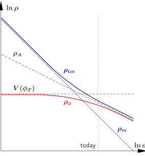
expect quintessence to unfreeze and start slow-rolling in an attempt to follow the tracker, as shown in Fig. 1. This however, is undermined by the fact that the tracker solution is losing its validity at present because we are no more in the pure matter era and the dark energy is about to dominate the Universe. Therefore, we should numerically investigate the problem, which may need a slightly modified value of M to work.

Preliminary study is optimistic and the resulting barotropic parameter for dark energy is within the observational bounds₋1_≤wφ≤ −0.95 [28].7 The same is true of its running.

In fact, the scenario presents some distinct observational signatures, because a potentially varying wφ is to be probed by forthcoming observations, such as EUCLID. We find that

φF ≥6.80mP and 0> wa ≥ −0.0659, wherewa≡ −dwφ/da|a=a0, (which is well within the

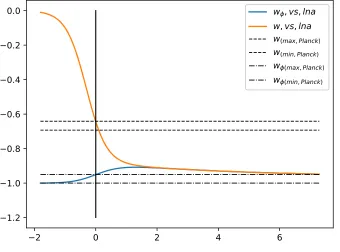
Planck bounds wa=−0.28+0₋0..2731 [28]), with ˆM = 6.25 TeV and a0 ≡a(t0) being the scale factor at the present time. The behaviour of the barotropic parameter of quintessence

wφ and of the Universe w is shown in Fig. 2 for the limiting case φF = 6.80mP (where

wa=−0.0659). We see that the values found satisfy the Planck bounds.

From Eq. (26), takingφF = 6.80mP corresponds to choosingQ= 0.002. Then, Eq. (12)

gives H = 1.16_×10−5_m

P. Using this, Eq. (13) suggests λ= 1.77×10−15. For the

infla-tionary observables, Eq. (16) results in ns = 0.967 and Eq. (14) gives r= 0.0130. Both

comfortably satisfy the observational bounds. The value ˆM = 6.25 TeV suggests that

M =λ−1/8_Mˆ _{= 4.36×10}5_{GeV. Finally, the potential density when the field is still frozen is}

V(φF) =

ˆ

M8

φ4 F

= (2.36×10−3_eV)4_{. (32)}

7

If quintessence were following the tracker solution in Eq. (28), then we would have

ln

ρ

ln

a

today

V

(

φ

)

ρ

ρ

ρ

ρ

Figure 1: Schematic log-log plot of the evolution of densities in thawing quintessence with

V(φ)∝φ−4_{. V(φ}

F) = constant is depicted with the horizontal dashed line. The attractor

(tracker)ρA∝a−2 is depicted with the slanted dot-dashed line. The slanted thin solid line

(blue) depicts the density of matterρm ∝a−3, while the lower thick solid line (red) depicts

ρφand the upper thick solid line (blue) depicts the total densityρtot =ρm+ρφ. The present

time is shown with the vertical dotted line. As evident in the figure, recently the density of quintessence unfreezes in an attempt to follow the tracker. Todayρm < ρφ< ρA< V(φF).

−2 0 2 4 6 −1.2

−1.0 −0.8 −0.6 −0.4 −0.2

0.0

w

vs

lna

w

vs

lna

w

w

w

w

Figure 2: Behaviour of the barotropic parameter of quintessencewφ(lower solid curve -blue)

and of the whole Universe w (upper solid curve - orange) as a function of the logarithm of the scale factor lna, which is normalised to unity today a0 = 1. We see that originally the Universe is in the matter era withw= 0 and the quintessence field is frozen with constant densityV(φF), such thatwφ=−1. However, when approaching the present time (depicted

by the vertical solid line - black) the quintessence unfreezes and wφ(t)>−1, while it also

begins to dominate the Universe so thatw(t)<0. Choosing the limiting caseφF = 6.80mP

the present values ofwφandw satisfy the Planck bounds, depicted by the horizontal lines.

In the future, quintessence becomes fully dominant sow_≈wφ, while it slow-rolls down the

quintessential tail of the scalar potential, ever more slowly, approximating w=wφ→ −1.

Comparing the above with ΩΛρ0as given in Eq. (27) we haveV(φF)/ΩΛρ0 = (2₂._.36₂₅)4 = 1.21>1, which agrees with the expectation that the field has unfrozen and its density at present is smaller than V(φF), as suggested by Fig. 1.

Before concluding, we briefly discuss the dissipative coefficient. By considering Υ6= Υ(φ) we implicitly considered the case when Υ =CTT, as in Ref. [25] (see also Ref. [30]). Then

we find

CT = 3QH/T . (33)

In order to have warm inflationT > H. Indeed, in Ref. [25] it is found thatT /H =_O(10). Thus, with Q= 0.002, Eq. (33) suggestsCT ∼10−3.

6

Conclusions

In this paper we have discussed warm quintessential inflation. As a toy model we have considered the original quintessential inflation model of Ref. [14], which is shown in Eq. (1). We stress however, that the scalar potential in Eq. (1) is only experienced during the inflation and quintessence regimes when _|φ_{| ∼}mP, while the field is kinetically dominated

when|φ| ≪mP, which means that it is oblivious of the potential, when crossing the origin.

Because of this fact, the exact form of the potential in Eq. (1) when|φ| ≪mP should not be

taken too seriously. In fact, warm quintessential inflation could in principle be a possibility when considering other models of quintessential inflation in the literature (see for example Ref. [12] and references therein).

The warm quintessential inflation model presented here appears promising for a more thorough investigation, especially of the time near the end of inflation and until reheating (which determinesN∗ and indirectly affects the inflationary observablesns andr) and also

of the time near the present, where there is connection with the dark energy observations. It is our intention to pursue this study, but we thought that the basic idea should be put out there first. Our promising findings suggest that modelling warm quintessential inflation can be a fruitful new avenue, especially when attempting to reconcile inflation, dark energy and the swampland conjectures.

Our paper appeared first but it was soon followed by Ref. [31], which studies a very similar model. There are aspects of the system studied where each paper focuses more than the other (for example, our work is more elaborate regarding the behaviour of the quintessence field at present) and, in that sense, both works complement each other.

References

[1] A. A. Starobinsky, Phys. Lett. B 91 (1980) 99 [Phys. Lett. 91B (1980) 99] [Adv. Ser. Astrophys. Cosmol. 3 (1987) 130]; K. Sato, Phys. Lett. 99B (1981) 66 [Adv. Ser. Astrophys. Cosmol. 3 (1987) 134]; D. Kazanas, Astrophys. J. 241 (1980) L59; A. H. Guth, Phys. Rev. D23(1981) 347 [Adv. Ser. Astrophys. Cosmol. 3(1987) 139].

[2] S. Perlmutter et al._{[Supernova Cosmology Project Collaboration], Astrophys. J. 517}

(1999) 565; A. G. Riess et al._{[Supernova Search Team], Astron. J. 116 (1998) 1009.}

[3] P. J. E. Peebles and B. Ratra, Rev. Mod. Phys. 75 (2003) 559; T. Padmanabhan, Phys. Rept. 380 (2003) 235; E. J. Copeland, M. Sami and S. Tsujikawa, Int. J. Mod. Phys. D 15 (2006) 1753.

[4] G. Obied, H. Ooguri, L. Spodyneiko and C. Vafa, arXiv:1806.08362 [hep-th]; H. Ooguri, E. Palti, G. Shiu and C. Vafa, Phys. Lett. B 788 (2019) 180.

[5] P. Agrawal, G. Obied, P. J. Steinhardt and C. Vafa, Phys. Lett. B784 (2018) 271;

[6] Y. Akrami, R. Kallosh, A. Linde and V. Vardanyan, Fortsch. Phys. 67(2019) no.1-2, 1800075.

[7] S. K. Garg and C. Krishnan, arXiv:1807.05193 [hep-th]; W. H. Kinney, S. Vagnozzi and L. Visinelli, Class. Quant. Grav. 36 (2019) no.11, 117001; A. Achcarro and G. A. Palma, JCAP 1902 (2019) 041; A. Kehagias and A. Riotto, Fortsch. Phys.

66 (2018) no.10, 1800052.

[8] S. Das, Phys. Rev. D 99 (2019) no.8, 083510; S. Das, Phys. Rev. D 99 (2019) no.6, 063514; M. Motaharfar, V. Kamali and R. O. Ramos, Phys. Rev. D 99 (2019) no.6, 063513.

[9] A. Berera, Phys. Rev. Lett. 75 (1995) 3218.

[10] C. Wetterich, Nucl. Phys. B 302 (1988) 668; B. Ratra and P. J. E. Peebles, Phys. Rev. D37 (1988) 3406; P. G. Ferreira and M. Joyce, Phys. Rev. D58 (1998) 023503; R. R. Caldwell, R. Dave and P. J. Steinhardt, Phys. Rev. Lett. 80 (1998) 1582.

[11] M. Cicoli, S. De Alwis, A. Maharana, F. Muia and F. Quevedo, Fortsch. Phys. 67

(2019) no.1-2, 1800079; L. Heisenberg, M. Bartelmann, R. Brandenberger and A. Re-fregier, Phys. Rev. D 98 (2018) no.12, 123502; Sci. China Phys. Mech. Astron. 62

(2019) no.9, 990421.

[13] M. W. Hossain, R. Myrzakulov, M. Sami and E. N. Saridakis, Phys. Rev. D 90

(2014) no.2, 023512; Phys. Rev. D 89 (2014) no.12, 123513; Int. J. Mod. Phys. D

24 (2015) no.05, 1530014; C. Q. Geng, M. W. Hossain, R. Myrzakulov, M. Sami and E. N. Saridakis, Phys. Rev. D 92 (2015) no.2, 023522.

[14] P. J. E. Peebles and A. Vilenkin, Phys. Rev. D 59 (1999) 063505.

[15] M. Giovannini, arXiv:1905.06182 [gr-qc]; . Haro, W. Yang and S. Pan, JCAP 1901

(2019) no.01, 023.

[16] R. J. Scherrer and A. A. Sen, Phys. Rev. D 77 (2008) 083515; T. Chiba, Phys. Rev. D 79 (2009) 083517 Erratum: [Phys. Rev. D 80 (2009) 109902].

[17] B. Spokoiny, Phys. Lett. B 315 (1993) 40; M. Joyce and T. Prokopec, Phys. Rev. D

57 (1998) 6022.

[18] L. H. Ford, Phys. Rev. D 35(1987) 2955; E. J. Chun, S. Scopel and I. Zaballa, JCAP

0907 (2009) 022.

[19] G. N. Felder, L. Kofman and A. D. Linde, Phys. Rev. D59(1999) 123523; A. H. Cam-pos, H. C. Reis and R. Rosenfeld, Phys. Lett. B 575 (2003) 151.

[20] B. Feng and M. z. Li, Phys. Lett. B564 (2003) 169; J. C. Bueno Sanchez and K. Di-mopoulos, JCAP 0711 (2007) 007.

[21] K. Dimopoulos and T. Markkanen, JCAP 1806 (2018) no.06, 021.

[22] T. Opferkuch, P. Schwaller and B. A. Stefanek, arXiv:1905.06823 [gr-qc].

[23] S. Ahmad, R. Myrzakulov and M. Sami, Phys. Rev. D 96 (2017) no.6, 063515.

[24] L. M. H. Hall, I. G. Moss and A. Berera, Phys. Rev. D 69 (2004) 083525; I. G. Moss and C. M. Graham, Phys. Rev. D 78 (2008) 123526; M. Bastero-Gil, A. Berera and R. O. Ramos, JCAP 1107 (2011) 030; R. O. Ramos and L. A. da Silva, JCAP 1303

(2013) 032.

[25] M. Bastero-Gil, S. Bhattacharya, K. Dutta and M. R. Gangopadhyay, JCAP 1802

(2018) no.02, 054.

[26] R. Arya, A. Dasgupta, G. Goswami, J. Prasad and R. Rangarajan, JCAP1802(2018) no.02, 043; M. Benetti and R. O. Ramos, Phys. Rev. D 95 (2017) no.2, 023517; S. Bartrum, M. Bastero-Gil, A. Berera, R. Cerezo, R. O. Ramos and J. G. Rosa, Phys. Lett. B 732 (2014) 116; M. Bastero-Gil, A. Berera and R. O. Ramos, JCAP

1107 (2011) 030; M. Bastero-Gil and A. Berera, Phys. Rev. D 76 (2007) 043515.

[28] Y. Akramiet al._{[Planck Collaboration], arXiv:1807.06211 [astro-ph.CO]; N. Aghanim} et al. _{[Planck Collaboration], arXiv:1807.06209 [astro-ph.CO].}

[29] P. J. Steinhardt, L. M. Wang and I. Zlatev, Phys. Rev. D59(1999) 123504; T. Chiba, A. De Felice and S. Tsujikawa, Phys. Rev. D 87 (2013) no.8, 083505; I. Zlatev, L. M. Wang and P. J. Steinhardt, Phys. Rev. Lett. 82 (1999) 896.

[30] M. Bastero-Gil, A. Berera, R. O. Ramos and J. G. Rosa, Phys. Rev. Lett.117 (2016) no.15, 151301; M. Bastero-Gil, A. Berera, R. Hernndez-Jimnez and J. G. Rosa, Phys. Rev. D 98 (2018) no.8, 083502.