which ran from November 30, 2016 to August 25, 2017, saw the first detection of gravitational waves from a binary neutron star inspiral, in addition to the observation of gravitational waves from a total of seven binary black hole mergers, four of which we report here for the first time: GW170729, GW170809, GW170818, and GW170823. For all significant gravitational-wave events, we provide estimates of the source properties. The detected binary black holes have total masses between 18.6þ−03..72M⊙ and
84.4þ−1115..18 M⊙ and range in distance between 320þ−110120 and 2840þ−13601400Mpc. No neutron star–black hole mergers were detected. In addition to highly significant gravitational-wave events, we also provide a list of marginal event candidates with an estimated false-alarm rate less than 1 per 30 days. From these results over the first two observing runs, which include approximately one gravitational-wave detection per 15 days of data searched, we infer merger rates at the 90% confidence intervals of110−3840Gpc−3y−1 for binary neutron stars and 9.7−101Gpc−3y−1 for binary black holes assuming fixed population distributions and determine a neutron star–black hole merger rate 90% upper limit of610Gpc−3y−1.
DOI:10.1103/PhysRevX.9.031040 Subject Areas: Astrophysics, Gravitation
I. INTRODUCTION
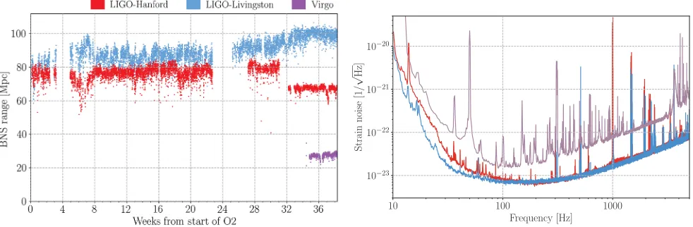
The first observing run (O1) of Advanced LIGO, which took place from September 12, 2015 until January 19, 2016, saw the first detections of gravitational waves (GWs) from stellar-mass binary black holes (BBHs) [1–4]. After an upgrade and commissioning period, the second observ-ing run (O2) of the Advanced LIGO detectors [5] com-menced on November 30, 2016 and ended on August 25, 2017. On August 1, 2017, the Advanced Virgo detector[6] joined the observing run, enabling the first three-detector observations of GWs. This network of ground-based interferometric detectors is sensitive to GWs from the inspiral, merger, and ringdown of compact binary coales-cences (CBCs), covering a frequency range from about 15 Hz up to a few kilohertz (see Fig.1). In this catalog, we report 11 confident detections of GWs from compact binary mergers as well as a selection of less significant triggers from both observing runs. The observations reported here and future GW detections will shed light on binary
formation channels, enable precision tests of general relativity (GR) in its strong-field regime, and open up new avenues of astronomy research.
The events presented here are obtained from a total of three searches: two matched-filter searches, PyCBC[7,8] and GstLAL[9,10], using relativistic models of GWs from CBCs, as well as one unmodeled search for short-duration transient signals or bursts, coherent WaveBurst (cWB)[11]. The two matched-filter searches target GWs from com-pact binaries with a redshifted total mass Mð1þzÞ of 2–500M⊙ for PyCBC and2–400M⊙for GstLAL, where zis the cosmological redshift of the source binary[12], and with maximal dimensionless spins of 0.998 for black holes (BHs) and 0.05 for neutron stars (NSs). The results of a matched-filter search for sub-solar-mass compact objects in
O1can be found in Ref. [13]; the results for O2will be discussed elsewhere. The burst search cWB does not use waveform models to compare against the data but instead identifies regions of excess power in the time-frequency representation of the gravitational strain. We report results from a cWB analysis that is optimized for the detection of compact binaries with a total mass less than 100M⊙.
A different tuning of the cWB analysis is used for a search for intermediate-mass BBHs with total masses greater than 100M⊙; the results of that analysis are discussed
else-where. The three searches reported here use different methodologies to identify GWs from compact binaries
*Full author list given at the end of the article.
Published by the American Physical Society under the terms of
the Creative Commons Attribution 4.0 International license.
in an overlapping but not identical search space, thus providing three largely independent analyses that allow for important cross-checks and yield consistent results. All searches have undergone improvements since O1, making it scientifically valuable to reanalyze theO1 data in order to reevaluate the significance of previously identified GW events and to potentially discover new ones. The searches identified a total of ten BBH mergers and one binary neutron star (BNS) signal. The GW events GW150914, GW151012 [14], GW151226, GW170104, GW170608, GW170814, and GW170817 have been reported previously[4,15–18]. In this catalog, we announce four previously unpublished BBH mergers observed during O2: GW170729, GW170809, GW170818, and GW170823. We estimate the total mass of GW170729 to be 84.4þ−1115..18 M⊙, making it the highest-mass BBH
observed to date. GW170818 is the second BBH observed in triple coincidence between the two LIGO observatories and Virgo after GW170814 [16]. As the sky location is primarily determined by the differences in the times of arrival of the GW signal at the different detector sites, LIGO-Virgo coincident events have a vastly improved sky localization, which is crucial for electromagnetic follow-up campaigns [19–22]. The reanalysis of the O1
data did not result in the discovery of any new GW events, but GW151012 is now detected with increased signifi-cance. In addition, we list 14 GW candidate events that have an estimated false-alarm rate (FAR) less than 1 per 30 days in either of the two matched-filter analyses but whose astrophysical origin cannot be established nor excluded unambiguously (Sec. VII).
Gravitational waves from compact binaries carry infor-mation about the properties of the source such as the masses and spins. These can be extracted via Bayesian inference by using theoretical models of the GW signal that describe the inspiral, merger, and ringdown of the final object for BBH
[23–30]and the inspiral (and merger) for BNS[31–33]. Such models are built by combining post-Newtonian calculations [34–38], the effective-one-body formalism [39–44], and numerical relativity[45–50]. Based on a variety of theoreti-cal models, we provide key source properties of all confident GW detections. For previously reported detections, we provide updated parameter estimates which exploit refined instrumental calibration, noise subtraction (for O2 data) [51,52], and updated amplitude power spectral density estimates[53,54].
The observation of these GW events allows us to place constraints on the rates of stellar-mass BBH and BNS mergers in the Universe and probe their mass and spin distributions, putting them into astrophysical context. The nonobservation of GWs from a neutron star–black hole binary (NSBH) yields a stronger 90% upper limit on the rate. The details of the astrophysical implications of our observations are discussed in Ref.[55].
This paper is organized as follows: In Sec. II, we provide an overview of the operating detectors duringO2, as well as the data used in the searches and parameter estimation. Section III briefly summarizes the three different searches, before we define the event selection criteria and present the results in Sec.IV. TablesIandII summarize some key search parameters for the clear GW detections and the marginal events. Details about the source properties of the GW events are given in Sec. V, and the values of some important parameters obtained from Bayesian inference are listed in TableIII. We do not provide parameter estimation results for marginal events. An independent consistency analysis between the waveform-based results and the data is performed in Sec.VI. In Sec.VII, we describe how the probability of astrophysical origin is calculated and give its value for each significant and marginal event in Table IV. We provide an updated estimate of binary merger rates in this
10 100 1000
Frequency [Hz] 10−23
10−22
10−21
10−20
Strain
noise
[1/
[image:2.612.62.553.50.211.2]√ Hz]
section before concluding in Sec.VIII. We also provide the Appendixes containing additional technical details.
A variety of additional information on each event, data products including strain data and posterior samples, and postprocessing tools can be obtained from the accompany-ing data release [56] hosted by the Gravitational Wave Open Science Center[57].
II. INSTRUMENTAL OVERVIEW AND DATA
A. LIGO instruments
The Advanced LIGO detectors[58,59]began scientific operations in September, 2015 and almost immediately
detected the first gravitational waves from the BBH merger GW150914.
BetweenO1andO2, improvements were made to both LIGO instruments. At LIGO-Livingston (LLO), a mal-functioning temperature sensor[60]was replaced immedi-ately after O1, contributing to an increase in the BNS range from approximately 60 Mpc to approximately 80 Mpc[61]. Other major changes included adding passive tuned mass dampers on the end test mass suspensions to reduce ringing up of mechanical modes, installing a new output Faraday isolator, adding a new in-vacuum array of photodiodes for stabilizing the laser intensity, installing GW170814 10∶30∶43.5 <1.25×10 <1.00×10 <2.08×10 16.3 15.9 17.2 GW170817 12∶41∶04.4 <1.25×10⁻⁵ <1.00×10⁻⁷ 30.9 33.0
GW170818 02∶25∶09.1 4.20×10⁻⁵ 11.3
[image:3.612.50.561.99.260.2]GW170823 13∶13∶58.5 <3.29×10⁻⁵ <1.00×10⁻⁷ 2.14×10⁻³ 11.1 11.5 10.8
TABLE II. Marginal triggers from the two matched-filter CBC searches. To distinguish events occurring on the same UTC day, we extend the YYMMDD label by decimal fractions of a day as needed, always rounding down (truncating) the decimal. The search that identifies each trigger is given, and the false alarm and network SNR. This network SNR is the quadrature sum of the individual detector SNRs for all detectors involved in the reported trigger; that can be fewer than the number of nominally operational detectors at the time, depending on the ranking algorithm of each pipeline. The detector chirp mass reported is that of the most significant template of the search. The concentration of our marginal triggers at low chirp masses is consistent with expectations for noise triggers, because search template waveforms are much more densely packed at low masses. The final column indicates whether there are any detector characterization concerns with the trigger; for an explanation and more details, see the text.
Date UTC Search FAR½y−1 Network SNR Mdet ½M
⊙ Data quality
151008 14∶09∶17.5 PyCBC 10.17 8.8 5.12 No artifacts
151012.2 06∶30∶45.2 GstLAL 8.56 9.6 2.01 Artifacts present
151116 22∶41∶48.7 PyCBC 4.77 9.0 1.24 No artifacts
161202 03∶53∶44.9 GstLAL 6.00 10.5 1.54 Artifacts possibly caused
161217 07∶16∶24.4 GstLAL 10.12 10.7 7.86 Artifacts possibly caused
170208 10∶39∶25.8 GstLAL 11.18 10.0 7.39 Artifacts present
170219 14∶04∶09.0 GstLAL 6.26 9.6 1.53 No artifacts
170405 11∶04∶52.7 GstLAL 4.55 9.3 1.44 Artifacts present
170412 15∶56∶39.0 GstLAL 8.22 9.7 4.36 Artifacts possibly caused
170423 12∶10∶45.0 GstLAL 6.47 8.9 1.17 No artifacts
170616 19∶47∶20.8 PyCBC 1.94 9.1 2.75 Artifacts present
170630 16∶17∶07.8 GstLAL 10.46 9.7 0.90 Artifacts present
170705 08∶45∶16.3 GstLAL 10.97 9.3 3.40 No artifacts
[image:3.612.54.561.372.548.2]higher quantum-efficiency photodiodes at the output port, and replacing the compensation plate on the input test mass suspension for theYarm. An attempt to upgrade the LLO laser to provide higher input power was not successful. During O2, improvements to the detector sensitivity con-tinued, and sources of scattered light noise were mitigated. As a result, the sensitivity of the LLO instrument rose from a BNS range of 80 Mpc at the beginning ofO2to greater than 100 Mpc by the run’s end.
The LIGO-Hanford (LHO) detector had a range of approximately 80 Mpc as O1 ended, and it was decided to concentrate on increasing the input laser power and forgo any incursions into the vacuum system. Increasing the input laser power to 50 W was successful, but since this increase did not result in an improvement in sensitivity, the LHO detector operated with 30 W input power duringO2. It was eventually discovered that there was a point absorber on one of the input test mass optics, which we speculate led to increased coupling of input “jitter” noise from the laser table into the interferometer. By use of appropriate witness sensors, it was possible to perform an offline noise subtraction on the data, leading to an increase in the BNS range at LHO by an average of about 20% over all of O2[51,52].
On July 6, 2017, LHO was severely affected by a 5.8 magnitude earthquake in Montana. Postearthquake, the sensitivity of the detector dropped by approximately 10 Mpc and remained in this condition until the end of the run on August 25, 2017.
B. Virgo instrument
Advanced Virgo[6]aims to increase the sensitivity of the Virgo interferometer by one order of magnitude, and several upgrades were performed after the decommission-ing of the first-generation detector in 2011. The main modifications include a new optical design, heavier mir-rors, and suspended optical benches, including photodiodes in a vacuum. Special care was also taken to improve the decoupling of the instrument from environmental disturb-ances. One of the main limiting noise sources below 100 Hz is the thermal Brownian excitation of the wires used for suspending the mirrors. A first test performed on the Virgo configuration showed that silica fibers would reduce this contribution. A vacuum contamination issue, which has since been corrected, led to failures of these silica suspen-sion fibers, so metal wires were used to avoid delaying Virgo’s participation inO2. Unlike the LIGO instruments, Virgo has not yet implemented signal recycling, which will be installed in a later upgrade of the instrument.
After several months of commissioning, Virgo joinedO2
on August 1, 2017 with a BNS range of approximately 25 Mpc. The performance experienced a temporary deg-radation on August 11 and 12, when the microseismic activity on site was highly elevated and it was difficult to keep the interferometer in its low-noise operating mode.
C. Data
Figure1shows the BNS ranges of the LIGO and Virgo instruments over the course ofO2and the representative amplitude spectral density plots of the total strain noise for each detector.
We subtract several independent contributions to the instrumental noise from the data at both LIGO detectors [51]. For all ofO2, the average increase in the BNS range from this noise subtraction process at LHO is approxi-mately 20% [51]. At LLO, the noise-subtraction process targeted narrow line features, resulting in a negligible increase in the BNS range.
Calibrated strain data from each interferometer are produced online for use in low-latency searches. Following the run, a final frequency-dependent calibration is gener-ated for each interferometer.
For the LIGO instruments, this final calibration benefits from the use of postrun measurements and the removal of instrumental lines. The calibration uncertainties are 3.8% in amplitude and 2.1° in phase for LLO and 2.6% in amplitude and 2.4° in phase for LHO. The results cited in this paper use the full frequency-dependent calibration uncertainties described in Refs.[64,65]. The LIGO timing uncertainty of
<1μs[66] is included in the phase correction factor. The calibration of strain data produced online by Virgo has large uncertainties due to the short time available for measurements. The data are reprocessed to reduce the errors by taking into account better calibration models obtained from postrun measurements and the subtraction of frequency noise. The reprocessing includes a time depend-ence for the noise subtraction and for the determination of the finesse of the cavities. The final uncertainties are 5.1% in amplitude and 2.3° in phase[67]. The Virgo calibration has an additional uncertainty of20μs originating from the time stamping of the data.
During O2, the individual LIGO detectors had duty factors of approximately 60% with a LIGO network duty factor of about 45%. Times with significant instrumental disturbances are flagged and removed, resulting in about 118 days of data suitable for coincident analysis[68]. Of these data, about 15 days are collected in coincident operation with Virgo, which after joiningO2operated with a duty factor of about 80%. Times with excess instrumental noise, which is not expected to render the data unusable, are also flagged[68]. Individual searches may then decide to include or not include such times in their final results.
III. SEARCHES
improvements made since their use in O1[4].
A. The PyCBC search
A pipeline to search for GWs from CBCs is constructed using the PyCBC software package [7,8]. This analysis performs direct matched filtering of the data against a bank of template waveforms to calculate the signal-to-noise ratio (SNR) for each combination of detector, template wave-form, and coalescence time [70]. Whenever the local maximum of this SNR time series is larger than a threshold of 5.5, the pipeline produces a single-detector trigger associated with the detector, the parameters of the template, and the coalescence time. In order to suppress triggers caused by high-amplitude noise transients (“glitches”), two signal-based vetoes may be calculated[71,72]. Using the SNR, the results of these two vetoes, and a fitting and smoothing procedure designed to ensure that the rate of single-detector triggers is approximately constant across the search parameter space, a single-detector rank ϱ is calculated for each single-detector trigger[73].
After generating triggers in the Hanford and Livingston detectors as described above, PyCBC finds two-detector coincidences by requiring a trigger from each detector associated with the same template and with coalescence times within 15 ms of each other. This time window accounts for the maximum light-travel time between LHO and LLO as well as the uncertainty in the inferred coalescence time at each detector. Coincident triggers are assigned a ranking statistic that approximates the relative likelihood of obtaining the event’s measured trigger param-eters in the presence of a GW signal versus in the presence of noise alone [73]. The detailed construction of this network statistic, as well as the single-detector rank ϱ, is improved from the corresponding statistics used in O1, partially motivating the reanalysis ofO1 by this pipeline. Finally, the statistical significances of coincident triggers are quantified by their inverse false-alarm rate (IFAR). This rate is estimated by applying the same coincidence pro-cedure after repeatedly time shifting the triggers from one detector and using the resulting coincidences as a back-ground sample. Each foreback-ground coincident trigger is
shifts within a given analysis period, which is done because the noise characteristics of the detector vary significantly from the beginning ofO1through the end of O2, so this restriction more accurately reflects the variation in detector performance. This restriction means, however, that the minimum bound on the false-alarm rate of candidates that have a higher ranking statistic than any trigger in the background sample is larger than it would be if longer periods of data are used for the time-shift analysis.
For the PyCBC analysis presented here, the template bank described in Ref. [75] is used. This bank covers binary systems with a total mass between 2 and500M⊙and mass
ratios down to1=98. Components of the binary with a mass below 2M⊙ are assumed to be neutron stars and have a
maximum spin magnitude of 0.05; otherwise, the maximum magnitude is 0.998. The high-mass boundary of the search space is determined by the requirement that the waveform duration be at least 0.15 s, which reduces the number of false-alarm triggers from short instrumental glitches. The waveform models used are a reduced-order-model (ROM) [29,76–78]of SEOBNRv4[29]for systems with a total mass greater than4M⊙ and TaylorF2[38,80]otherwise.
B. The GstLAL search
only noise is present [9,82,83]. The noise model is constructed, in part, from single-detector triggers that are not found in coincidence, so as to minimize the possibility of contamination by real signals. In the search presented here, the likelihood ratio is a function of ρ, a signal-consistency test, the differences in time and phase between the coincident triggers, the detectors that contribute triggers to the candidate, the sensitivity of the detectors to signals at the time of the candidate, and the rate of triggers in each of the detectors at the time of the candidate[9]. This function is an expansion of the parameters used to model the likelihood ratio in earlier versions of GstLAL and improves the sensitivity of the pipeline used for this search over that used in O1.
The GstLAL search uses Monte Carlo methods and the likelihood ratio’s noise model to determine the probability of observing a candidate with a log likelihood ratio greater than or equal to logL, PðlogL≥logLjnoiseÞ. The expected number of candidates from noise with log likelihood ratios at least as high as logL is then
NPðlogL≥logLjnoiseÞ, where N is the number of observed candidates. The FAR is then the total number of expected candidates from noise divided by the live time of the experiment, T, and the p value is obtained by assuming the noise is a Poisson process:
FAR¼NPðlogL
≥logLjnoiseÞ
T ; ð2Þ
p¼1−e−NPðlogL≥logLjnoiseÞ: ð3Þ
For the analysis in this paper, GstLAL analyzes the same periods of data as PyCBC. However, FARs are assigned using the distribution of likelihood ratios in noise computed from marginalizing PðlogL≥logLjnoise;periodÞ over all analysis periods; thus, all of O1 and O2 are used to inform the noise model for FAR assignment. The only exception is GW170608. The analysis period used to estimate the significance of GW170608 is unique from the other ones[17], and thus its FAR is assigned using only its local background statistics.
For this search, GstLAL uses a bank of templates with a total mass between 2 and400M⊙and a mass ratio between
1=98and 1. Components with a mass less than2M⊙have
a maximum spin magnitude of 0.05 (as for PyCBC); otherwise, the spin magnitude is less than 0.999. The TaylorF2 waveform approximant is used to generate templates for systems with a chirp mass [see Eq.(5)] less than 1.73, and the reduced-order model of the SEOBNRv4 approximant is used elsewhere. More details on the bank construction can be found in Ref.[84].
C. Coherent WaveBurst
Coherent WaveBurst (cWB) is an analysis algorithm used in searches for weakly modeled (or unmodeled)
transient signals with networks of GW detectors. Designed to operate without a specific waveform model, cWB identifies coincident excess power in the multiresolution time-frequency representations of the detector strain data [85], for signal frequencies up to 1 kHz and durations up to a few seconds. The search identifies events that are coherent in multiple detectors and reconstructs the source sky location and signal waveforms by using the constrained maximum likelihood method [11]. The cWB detection statistic is based on the coherent energy Ec obtained by cross-correlating the signal waveforms reconstructed in the two detectors. It is proportional to the coherent network SNR and used to rank each cWB candidate event. For an estimation of its statistical significance, each candidate event is ranked against a sample of background triggers obtained by repeating the analysis on time-shifted data, similar to the background estimation in the PyCBC search. To exclude astrophysical events from the background sample, the time shifts are selected to be much larger than the expected signal delay between the detectors. Each cWB event is assigned a FAR given by the rate of background triggers with a larger coherent network SNR.
To increase robustness against nonstationary detector noise, cWB uses signal-independent vetoes, which reduce the high rate of the initial excess power triggers. The primary veto cut is on the network correlation coefficient
cc ¼Ec=ðEcþEnÞ, whereEn is the residual noise energy estimated after the reconstructed signal is subtracted from the data. Typically, for a GW signal cc≈1, and for instrumental glitchescc≪1. Therefore, candidate events withcc<0.7are rejected as potential glitches.
Finally, to improve the detection efficiency for a specific class of stellar-mass BBH sources and further reduce the number of false alarms, cWB selects a subset of detected events for which the frequency is increasing with time, i.e., events with a chirping frequency pattern. Such a time-frequency pattern captures the phenomenological behavior of most CBC sources. This flexibility allows cWB to potentially identify CBC sources with features such as higher-order modes, high mass ratios, misaligned spins, and eccentric orbits; it complements the existing templated algorithms by searching for new and possibly unexpected CBC populations. For events that passed the signal-independent vetoes and chirp cut, the detection significance is characterized by a FAR computed as described above; otherwise, cWB provides only the reconstructed waveforms (see Sec.VI).
IV. SEARCH RESULTS
A. Selection criteria
independent noise events, we would expect on average two such noise events (false alarms) per month of analyzed coincident time. During these first two observing runs, we also empirically observe approximately two likely signal events per month of analyzed time. Thus, forO1andO2, any sample of events all of whose measured FARs are greaterthan 1 per 30 days is expected to consist of at least 50% noise triggers. Individual triggers within such a sample are then considered to be of little astrophysical interest. Since the number of triggers with a FAR less than 1 per 30 days is manageable, restricting our attention to triggers with lower FAR captures all confident detections while also probing noise triggers.
Within the sample of triggers with a FAR less than the ceiling of 1 per 30 days in at least one of the matched-filter searches, we assign the“GW”designation to any event for which the probability of astrophysical origin from either matched-filter search is greater than 50% (for the exact
function of the inverse false-alarm rate, as well as the expected background for the analysis time, with Poisson uncertainty bands. The foreground distributions clearly stand out from the background, even though we show only rightward-pointing arrows for any event with a measured or bounded IFAR greater than 3000 y.
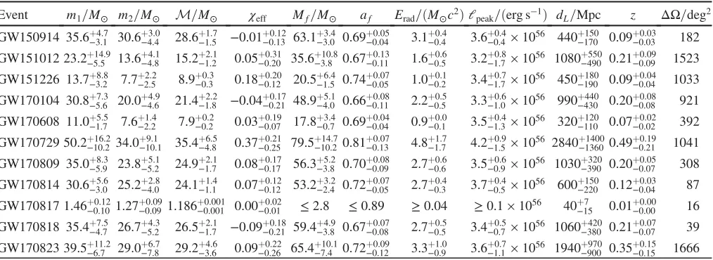
We present more quantitative details below on the 11 gravitational events, as selected by the criteria in Sec.IVA, in TableI. Of these 11 events, seven have been previously reported: the three gravitational-wave events fromO1[1–4] and, fromO2, the binary neutron star merger GW170817 [18] and the binary black hole events GW170104 [15], GW170608[17], and GW170814[16]. The updated results we report here supersede those previously published. Four new gravitational-wave events are reported here for the first time: GW170729, GW170809, GW170818, and GW170823. All four are binary black hole events.
[image:7.612.62.559.456.665.2]As noted in Sec. III, data from O1 are reanalyzed because of improvements in the search pipelines and the
expansion of the parameter space searched. For the O2
events already published, our reanalysis is motivated by updates to the data itself. The noise subtraction procedure [52]that is available for parameter estimation of three of the publishedO2events was not initially applied to the entire
O2dataset and, therefore, could not be used by searches. Following the procedures of Ref. [51], this noise subtrac-tion is applied to all ofO2and is reflected in TableIfor the four previously published O2GW events, as well as the four events presented here for the first time.
For both PyCBC and cWB, the time-shift method of background estimation may result in only an upper bound on the false-alarm rate, if an event has a larger value of the ranking statistic than any trigger in the time-shifted back-ground; this result is indicated in TableI. For GW150914 and GW151226, the bound that PyCBC places on the FAR in these updated results is in fact higher than that previously published [1,2,4], because, as noted in Sec. III A, this search elects to use shorter periods of time shifting to better capture the variation in the detectors’ sensitivities. For GstLAL, the FAR is reported in TableIas an upper bound of 1.00×10⁻⁷ whenever a smaller number is obtained, which reflects a more conservative noise hypothesis within the GstLAL analysis and follows the procedures and motivations detailed in Sec. IV in Ref.[3].
Five of the GW events reported here occurred during August 2017, which comprises approximately 10% of the total observation time. There are ten nonoverlapping periods of similar duration, with an average event rate of 1.1 per
period. The probability that a Poisson process would produce five events or more in at least one of those periods is 5.3%. Thus, seeing five events in one month is statistically consistent with expectations. For more details, see Ref.[87]. For the remainder of this section, we briefly discuss each of the gravitational-wave events, highlighting interesting fea-tures from the perspectives of the three searches. A discussion of the properties of these sources may be found in Sec.V. Though the results presented are from the final, offline analysis of each search, for the four new GW events, we also indicate whether the event is found in a low-latency search and an alert sent to electromagnetic observing partners. Where this process did occur, we mention in this paper only the low-latency versions of the three searches with offline results presented here; in some cases, additional low-latency pipelines also found events. A more thorough discussion of all of the low-latency analyses and the electromagnetic follow-up ofO2events may be found in Ref.[22].
1. GW150914, GW151012, and GW151226
During O1, two confident detections of binary black holes were made: GW150914 [1] and GW151226 [2]. Additionally, a third trigger was noted in theO1catalog of binary black holes[3,4]and labeled LVT151012. That label is a consequence of the higher FAR of that trigger, though detector characterization studies show no instrumental or environmental artifact, and the results of parameter esti-mation are consistent with an astrophysical BBH source. Even with the significance that is measured with the
O1 search pipelines [4], this event meets the criteria of Sec.IVAfor a gravitational-wave event, and we henceforth relabel this event as GW151012.
The improvedO2pipelines substantially reduce the FAR assigned to GW151012: It is now0.17y−1in the PyCBC search (previously, 0.37y−1) and 7.92×10⁻³y−1 in the GstLAL search (previously, 0.17y−1). These improved FAR measurements for GW151012 are the most salient result of the reanalysis ofO1with theO2pipelines; no new gravitational-wave events were discovered. The first binary black hole observation, GW150914, remains the highest SNR event inO1and the second highest in the combined
O1and O2 datasets, behind only the binary neutron star inspiral GW170817.
Recently, Ref.[88]appeared. That catalog also presents search results from the PyCBC pipeline forO1 and also finds GW150914, GW151012, and GW151226 as the only confident gravitational-wave events inO1, with iden-tical bounds on FAR to the PyCBC results in TableI for GW150914 and GW151226. The measured FAR for GW151012 is not identical but is consistent with the results we present in TableI.
2. GW170104, GW170608, and GW170814
[image:8.612.54.296.45.247.2]Three binary black hole events from O2have already been published: GW170104 [15], GW170608[17], and FIG. 3. Cumulative histograms of search results for the cWB
GstLAL. This results from the noise subtraction in the LIGO data and updated calibration of the Virgo data. Because of the noise subtraction in the LIGO data, under GstLAL’s ranking of multiple triggers[9], a new template generates the highest ranked trigger as double coincident, with a Hanford SNR of 9.1 (the previous highest ranked trigger, a triple, had 7.3). Though this highest ranked event is a double-coincident trigger, the pipeline does identify other highly significant triggers, some double coincident and some triple coincident. As the search uses a discrete template bank, peaks from the SNR time series of the individual detectors, and clustering of several coincident triggers over the bank, it is difficult in this case to tell from the search results alone whether the event is truly a triple-coincident detection. For a definitive answer, we perform a fully Bayesian analysis with and without the Virgo data, similar to the results in Ref. [16]. Comparing the evidence, this Bayesian analysis—which enforces coherence and therefore more fully exploits consistency among detected amplitudes, phases, and times of arrival than the search pipelines—finds that a triple-coincident detection is strongly favored over a double-coincident detection, by a factor of approximately 60. Thus, the updated results are consistent with those that were previously published.
3. GW170817
Across the entirety of O1 andO2, the binary neutron star inspiral GW170817 remains the event with the highest network SNR and is accordingly assigned the most stringent possible bound on its FAR by PyCBC and the highest value ofL(the logarithm of the likelihood ratio) of any event in the combinedO1andO2dataset by GstLAL. As explained in detail in the original detection paper[18], a loud glitch occurs near the end of this signal in LLO. For the matched-filter searches, this glitch is excised via time-domain gating (and that gating is applied consistently to all such glitches throughout O2). Because the cWB pipeline is designed to detect short signals, it does not use that gating technique, and it rejects this event because of the glitch.
between the PyCBC pipeline and cWB, using software injections with parameters drawn from the SEOBNRv4 ROM parameter estimation of this event. That waveform doesnotincorporate precession or higher-order modes, but, by using these samples as inputs to both searches, we can probe how often we see comparable results. It is found that approximately 4% of these SEOBNRv4 ROM samples are recovered by both the PyCBC and cWB pipelines with FAR≥1y−1and FAR≤0.02y−1, respectively. Thus, the observed difference in FARs between the two pipelines is not exceptionally unlikely and is consistent with a noise fluctuation which happens to decrease the significance of the event as seen by PyCBC and increase it for cWB. The detailed CBC parameter estimation studies in Sec.Valso indicate no significant evidence for observationally impor-tant precession or higher-order modes. This event was identified only in the offline analyses, so no alert was sent to electromagnetic partners.
5. GW170809
GW170809 was observed on August 9, 2017 at 08∶28∶21.8 UTC with a FAR of 1.45×10⁻⁴y−1 by PyCBC and <1.00×10⁻⁷ y−1 by GstLAL. This event was identified in low latency by both the GstLAL and cWB pipelines, and an alert was sent to electromagnetic observ-ing partners. In the final offline cWB analysis with updated calibration and noise subtracted from LIGO data, this event did not pass one of the signal-independent vetoes (Sec.III C) and was therefore not assigned a FAR.
6. GW170818
those of GstLAL and, therefore, well below the threshold of 5.5 needed for a single-detector trigger in the PyCBC search to be considered further for possible coincidence. This event is initially identified in low latency by the GstLAL pipeline as a LLO-Virgo double-detector trigger. Online, the Virgo trigger is not included in significance estimation, and the LLO-only trigger does not pass the false-alarm threshold for the online search. Therefore, at that time no alerts was sent to electromagnetic observing partners.
7. GW170823
On August 23, 2017, GW170823 was observed at 13∶13∶58.5 UTC. Its FAR is <3.29×10⁻⁵ y−1 in the PyCBC pipeline,<1.00×10⁻⁷ y−1in the GstLAL pipeline, and2.14×10−3y−1in the cWB pipeline. The online versions of each of these pipelines detect this event in low latency, and an alert is sent to electromagnetic observing partners.
C. Marginal triggers and instrumental artifacts
In TableII, we present the remaining 14 triggers fromO1
andO2that pass the initial threshold of a FAR less than one per 30 days in at least one of the two matched-filter searches but are not assigned a probability of astrophysical origin of more than 50% by either pipeline (see TableIV). As noise triggers are generically a function of the details of the pipeline that identifies a trigger, we do not typically expect to see the same noise triggers in each pipeline. In Table II, we therefore present which of the two pipelines identified the trigger, as well as the FAR of that trigger, its SNR, and the chirp mass of the template generating the trigger; these chirp masses do not come from a detailed parameter estimation as is performed in Sec. V for the gravitational-wave events.
Before discussing the final column in Table II, we consider the reasonableness of the number of these triggers. The matched-filter pipelines analyze 0.46 y of coincident data, so, at a false-alarm threshold of once per 30 days, we would expect about six triggers purely from noise. We see from Table II that the PyCBC search observed three marginal triggers and the GstLAL search observed 11. Though the probability that 11 triggers could arise only from noise when six are expected is low, it is by itself not sufficiently low to confidently assert that some fraction of these triggers are astrophysical in origin. It is possible, however, that either search’s marginal triggers could con-tain a population of real GW signals. In particular, the multicomponent population analysis[89,90](see Sec.VII) explicitly considers the possibility of triggers (both con-fident detections and marginal triggers) arising from a combination of noise and distinct source populations. For GstLAL, the combined count of GWs and marginal triggers is 22, and the analysis in Sec.VII finds that to be within expectations at the 90% level. Although it may be the case
that some of these marginal triggers are of astrophysical origin, we cannot then determine which ones.
Now we turn to a summary of the detector characteri-zation information for each marginal trigger, briefly indi-cated in the final column in TableII. Following a subset of procedures used for previous gravitational-wave detections [91], we evaluate the possibility that artifacts from instru-mental or environinstru-mental noise could have caused each of the marginal triggers. Using auxiliary sensors at each detector, as well as the gravitational-wave strain data, we evaluate the state of the detectors at the time of each marginal trigger, identify and investigate any artifacts in the data due to noise, and test whether any identified artifacts might explain the excess SNR observed in the analysis. Of the marginal triggers presented in this catalog, nine have excess power from known sources of noise occurring during times when the matched-filter template that yields the trigger has a GW frequency within the sensitive band of the detectors. For four of these cases, the observed instrumental artifact overlaps the signal region and possibly causes the marginal trigger.
Details on the physical couplings that create these instrumental artifacts and possible mitigation strategies useful for analysis of LIGO-Virgo data are discussed in Appendix A. For the remainder of this subsection, we describe how the different categories discussed in that Appendix apply to the marginal triggers in TableII.
To determine whether artifacts identified as noise “could account for”marginal triggers, we use two metrics: (i) whether the type of noise has been shown to produce an excess of triggers consistent with the properties of the trigger present and (ii) the noise artifact could account for the presence of the trigger as reported by that search, including SNR and time-frequency evolution, without the presence of an astrophysical signal.
In and of themselves, these classifications do not affect the probability that any particular marginal trigger is associated with a signal as measured by the searches but are statements about the evidence of transient noise in the detectors. It is expected that a substantial fraction of marginal events at the false-alarm rate values reported are caused by noise, given the estimated background of our searches and the expected rate of signals. See Sec. VII, Fig. 11, and Table IV below for a more detailed discussion of the probabilities of astrophysical or noise origin of such events.
1. No noise artifacts present: 151008, 151116, 170219, 170423, and 170705
Investigations into this set of marginal triggers have identified no instrumental artifacts in time coincidence with the triggers.
2. Light scattering possibly caused: 161217 and 170720
high-amplitude ground motion at Livingston caused by storm activity. During this storm activity, the Livingston detector is not able to maintain a stable interferometer for periods longer than 10 min. The presence of intense scattering artifacts contribute to the unstable state of the interferometer and could account for the SNR of the marginal trigger. Because of the short observing duration, this time period is not analyzed by the PyCBC search.
Within 20 s of trigger 170720, excess ground motion from earthquakes forced the Livingston detector to drop out of its nominal mode of operation. Before the detector dropped out of the observing state, the data are heavily polluted with scattering artifacts that could account for the SNR of the triggers. As the PyCBC search does not consider times near the edges of observing periods, this time period is also not analyzed by that search. Artifacts related to scattered light are also observed at Hanford at this time.
3. Light scattering present: 151012.2, 170208, and 170616
In the case of trigger 151012.2, light scattering does not introduce significant power above 30 Hz prior to the reported trigger time. Investigations into the relationship between the trigger and the scattered light find no power overlap, suggesting that the artifacts could not account for the observed marginal trigger.
Investigations into triggers 170208 and 170616 find similar results. In the case of these triggers, a slight overlap with excess power from scattering is observed. Multiple efforts, including BAYESWAVE[53] glitch subtraction and
gating[8], are used to mitigate the scattered light artifacts. After subtraction of the noise artifacts, the data are reanalyzed to evaluate whether the excess power subtracted could have accounted for the trigger. In both cases, the marginal trigger remains with similar significance, sug-gesting that the observed scattering artifact could not have accounted for the SNR of the marginal trigger.
4. 60–200 Hz nonstationarity possibly caused: 161202 and 170412
This class of marginal triggers occurs during periods of noise referred to as “60–200 Hz nonstationarity.” This
170405 and 170630
The marginal triggers in this class occur in time coincidence with short-duration, high-amplitude noise transients that are removed in the data-conditioning step of the search pipelines [8]. The times surrounding these transients do not demonstrate an elevated trigger rate after the transient has been removed. Trigger 170405 is in coincidence with this class of transient at Hanford, and trigger 170630 is in coincidence with this class of transient at Livingston. As triggers 170405 and 170630 are identified as significant after the removal of the short-duration transients, the presence of noise artifacts cannot account for the SNR of these marginal triggers.
V. SOURCE PROPERTIES
Here, we present inferred source properties of gravita-tional-wave signals observed by the LIGO and Virgo detectors under the assumption that they originate from compact binary coalescences described by general rela-tivity. We analyze all GW events described in Sec. IV. Full parameter estimation (PE) results for O1 events are provided for GW150914 in Refs.[4,95,96], for GW151226 in Refs.[2,4], and for GW151012 in Refs.[3,4]. PE results for fourO2events are provided for GW170104 in Ref.[15], for GW170608 in Ref.[17], for GW170814 in Ref.[16], and for GW170817 in Refs.[18,97]. Data from the three-detector LIGO-Virgo network are used to obtain parameter estimates for GW170729, GW170809, GW170814, GW170817, and GW170818. Virgo data for GW170729, from the commis-sioning phase before it officially joined, are included for PE analyses, because the calibration of the data and the sensitivity of the instrument are comparable to that in August. For the remaining events, the analysis uses data from the two LIGO detectors.
We perform a reanalysis of the data for the entirety ofO1
and calibration have not changed, a reanalysis is valuable for the following reasons: (i) Parameter estimation analyses use an improved method for estimating the power spectral density of the detector noise[53,54]and frequency-depen-dent calibration envelopes[98]; (ii) we use two waveform models that incorporate precession and combine their posteriors to mitigate model uncertainties.
Key source parameters for the ten BBHs and one BNS are shown in TableIII. We quote the median and symmetric 90% credible intervals for inferred quantities. For BBH coales-cences, parameter uncertainties include statistical and sys-tematic errors from averaging posterior probability distributions over the two waveform models, as well as calibration uncertainty. Apart from GW170817, all posterior distributions of GW events are consistent with originating from BBHs. Posterior distributions for all GW events are shown in Figs. 4–8. Mass and tidal deformability poste-riors for GW170817 are shown in Fig. 9. For BBH coalescences, we present combined posterior distributions from an effective precessing spin waveform model (IMRPhenomPv2) [25,26,49] and a fully precessing model (SEOBNRv3) [27,28,30]. For the analysis of GW170817, we present results for three frequency-domain models IMRPhenomPv2NRT [25,26,32,49,99], SEOBNRv4NRT [29,32,77,99], and TaylorF2 [35,36, 38,100–112]and two time-domain models SEOBNRv4T [31] and TEOBResumS [33,113]. Details on Bayesian parameter estimation methods, prior choices, and wave-form models used for BBH and BNS systems are provided in AppendixB,B 1, andB 2, respectively. We discuss an
analysis including higher harmonics in the waveform in AppendixB 3and find results broadly consistent with the analysis presented below. The impact of prior choices on selected results is discussed in Appendix C.
A. Source parameters
The GW signal emitted from a BBH coalescence depends on intrinsic parameters that directly characterize the binary’s dynamics and emitted waveform, and extrinsic parameters that encode the relation of the source to the detector network. In general relativity, an isolated BH is uniquely described by its mass, spin, and electric charge [114–118]. For astrophysical BHs, we assume the electric charge to be negligible. A BBH undergoing quasicircular inspiral can be described by eight intrinsic parameters, the two massesmi, and the two three-dimensional spin vectors
⃗
Siof its component BHs defined at a reference frequency. Seven additional extrinsic parameters are needed to describe a BH binary: the sky location (right ascension α and declination δ), luminosity distance dL, the orbital inclinationιand polarization angleψ, the timetc, and phase ϕc at coalescence.
Since the maximum spin a Kerr BH of mass m can reach is ðGm2Þ=c, we define dimensionless spin vectors ⃗χi¼cS⃗ i=ðGm2iÞand spin magnitudesai¼cjS⃗ ij=ðGm2iÞ. If the spins have a component in the orbital plane, then the binary’s orbital angular momentumL⃗ and its spin vectors precess [119,120] around the total angular momentum
⃗
[image:12.612.54.561.153.338.2]J¼L⃗ þS⃗ 1þS⃗ 2.
TABLE III. Selected source parameters of the 11 confident detections. We report median values with 90% credible intervals that include statistical errors and systematic errors from averaging the results of two waveform models for BBHs. For GW170817, credible intervals and statistical errors are shown for IMRPhenomPv2NRT with a low spin prior, while the sky area is computed from TaylorF2 samples. The redshift for NGC 4993 from Ref.[94] and its associated uncertainties are used to calculate source-frame masses for GW170817. For BBH events, the redshift is calculated from the luminosity distance and assumed cosmology as discussed in AppendixB. The columns show source-frame component massesmiand chirp massM, dimensionless effective aligned spinχeff, final source-frame massMf, final spinaf, radiated energyErad, peak luminositylpeak, luminosity distancedL, redshiftz, and sky localization
ΔΩ. The sky localization is the area of the 90% credible region. For GW170817, we give conservative bounds on parameters of the final remnant discussed in Sec.V E.
Event m1=M⊙ m2=M⊙ M=M⊙ χeff Mf=M⊙ af Erad=ðM⊙c2Þlpeak=ðerg s−1Þ dL=Mpc z ΔΩ=deg2
GW150914 35.6þ−34..17 30.6þ−43..40 28.6−þ11..57 −0.01þ−00..1312 63.1þ−33..04 0.69þ−00..0405 3.1þ−00..44 3.6−þ00..44×1056 440−þ170150 0.09þ−00..0303 182 GW15101223.2þ14.9
−5.5 13.6
þ4.1
−4.8 15.2−þ12..21 0.05þ−00..2031 35.6þ−310.8.80.67þ−00..1113 1.6þ−00..56 3.2
þ0.8
−1.7×1056 1080þ−490550 0.21þ−00..0909 1523 GW151226 13.7þ−38..28 7.7þ−22..52 8.9−þ00..33 0.18þ−00..1220 20.5þ−16..54 0.74þ−00..0507 1.0þ−00..21 3.4−þ01..77×1056 450−þ190180 0.09þ−00..0404 1033 GW170104 30.8þ7.3
−5.6 20.0
þ4.9
−4.6 21.4−þ12..82 −0.04þ−00..2117 48.9þ−45..01 0.66þ−00..1108 2.2þ−00..55 3.3
þ0.6
−1.0×1056 990þ−430440 0.20þ−00..0808 921 GW170608 11.0þ−15..75 7.6þ−21..24 7.9−þ00..22 0.03þ−00..0719 17.8þ−03..74 0.69þ−00..0404 0.9þ−00..10 3.5−þ01..34×1056 320−þ110120 0.07þ−00..0202 392 GW17072950.2þ16.2
−10.2 34.0−þ109.1.1 35.4þ−46..85 0.37þ−00..2521 79.5
þ14.7
−10.2 0.81−þ00..1307 4.8þ−11..77 4.2þ−01..59×1056 2840
þ1400
−1360 0.49þ−00..2119 1041 GW170809 35.0þ−58..93 23.8þ−55..21 24.9−þ12..71 0.08þ−00..1717 56.3þ−35..82 0.70þ−00..0908 2.7þ−00..66 3.5−þ00..96×1056 1030−þ390320 0.20þ−00..0705 308 GW170814 30.6þ5.6
−3.0 25.2−þ42..08 24.1þ−11..14 0.07þ−00..1212 53.2þ−23..42 0.72þ−00..0507 2.7
þ0.4
−0.3 3.7þ−00..54×1056 600
þ150
−220 0.12þ−00..0403 87 GW1708171.46−þ00..10121.27þ−00..09091.186−þ00..001001 0.00−þ00..0102 ≤2.8 ≤0.89 ≥0.04 ≥0.1×1056 40−þ157 0.01−þ00..0000 16 GW170818 35.4þ7.5
−4.7 26.7þ−54..23 26.5
þ2.1
−1.7 −0.09−þ00..2118 59.4þ−34..89 0.67þ−00..0807 2.7þ−00..55 3.4
þ0.5
We describe the dominant spin effects by introducing effective parameters. The effective aligned spin is defined as a simple mass-weighted linear combination of the spins [23,24,121]projected onto the Newtonian angular momen-tumLˆN, which is normal to the orbital plane (Lˆ ¼LˆN for aligned-spin binaries)
χeff ¼
ðm1⃗χ1þm2⃗χ2Þ·LˆN
M ; ð4Þ
whereM¼m1þm2is the total mass of the binary andm1is
defined to be the mass of the larger component of the binary, such thatm1≥m2. Different parameterizations of spin effects
are possible and can be motivated from their appearance in the GW phase or dynamics [122–124]. χeff is approximately
conserved throughout the inspiral[121]. To assess whether a binary is precessing, we use a single effective precession spin parameterχp[125](see AppendixC).
During the inspiral, the phase evolution depends at leading order on the chirp mass[34,126,127]
M¼ðm1m2Þ3=5
M1=5 ; ð5Þ
which is also the best measured parameter for low-mass systems dominated by the inspiral [63,101,122,128]. The mass ratio
q¼m2
m1≤1 ð
6Þ
and effective aligned spin χeff appear in the phasing at higher orders [101,121,123].
For precessing binaries, the orbital angular momentum vector L⃗ is not a stable direction, and it is preferable to describe the source inclination by the angle θJN between
the total angular momentumJ⃗ (which typically is approx-imately constant throughout the inspiral) and the line-of-sight vector N⃗ instead of the orbital inclination angle ι between L⃗ and N⃗ [119,129]. We quote frequency-dependent quantities such as spin vectors and derived quantities asχpat a GW reference frequencyfref¼20Hz. Binary neutron stars have additional degrees of freedom (d.o.f.) related to their response to a tidal field. The dominant quadrupolar (l¼2) tidal deformation is described by the dimensionless tidal deformability Λ¼ ð2=3Þk2½ðc2=GÞðR=mÞ5of each neutron star (NS), where k2is the dimensionlessl¼2Love number andRis the NS
radius. The tidal deformabilities depend on the NS mass
m and the equation of state (EOS). The dominant tidal contribution to the GW phase evolution is encapsulated in an effective tidal deformability parameter[130,131]:
˜
Λ¼16
13
ðm1þ12m2Þm41Λ1þ ðm2þ12m1Þm42Λ2
M5 : ð7Þ
B. Masses
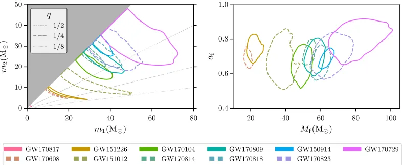
In the left panel in Fig. 4, we show the inferred component masses of the binaries in the source frame as contours in them1-m2plane. Because of the mass prior, we
consider only systems with m1≥m2 and exclude the
shaded region. The component masses of the detected BH binaries cover a wide range from about5M⊙to about
70M⊙ and lie within the range expected for stellar-mass
approximately 60–120M⊙ [135–138]. The lowest-mass
BBH systems, GW151226 and GW170608, have 90% credible lower bounds on m2 of 5.6M⊙ and 5.9M⊙,
respectively, and therefore lie above the proposed BH mass gap region[139–142]of2–5M⊙. The component masses
of the BBHs show a strong degeneracy with each other. Lower-mass systems are dominated by the inspiral of the binary, and the component mass contours trace out a line of constant chirp mass Eq. (5) which is the best measured parameter in the inspiral [34,63,122]. Since higher-mass systems merge at a lower GW frequency, their GW signal is dominated by the merger of the binary. For high-mass binaries, the total mass can be measured with an accuracy comparable to that of the chirp mass[143–146].
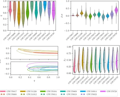
We show posteriors for the ratio of the component masses Eq. (6) in the top left in Fig.5. This parameter is much harder to constrain than the chirp mass. The width of the posteriors depends mostly on the SNR, and so the mass ratio is best measured for the loudest events, GW170817, GW150914, and GW170814. Even
though GW170817 has the highest SNR of all events, its mass ratio is less well constrained, because the signal power comes predominantly from the inspiral, while the merger contributes little compared to the BBH[147]. GW151226 and GW151012 have posterior support for more unequal mass ratios than the other events, with lower bounds of 0.28 and 0.29, respec-tively, at 90% credible level.
The final mass, radiated energy, final spin, and peak luminosity of the BH remnant from a BBH coalescence are computed using averages of fits to numerical relativity (NR) results[15,148–153]. Posteriors for the mass and spin of the BH remnant for BBH coalescences are shown in the right in Fig.4. Only a fractionð0.02–0.07Þof the binary’s total mass is radiated away in GWs. The amount of radiated energy scales with its total mass. The heaviest remnant BH found is GW170729, at 79.5þ−1014..27 M⊙ while the lightest
remnant BH is GW170608, at17.8þ−03..74M⊙.
[image:14.612.110.506.47.367.2]FIG. 7. Parameter estimation summary plots IV. Posterior probability densities of distancedL, inclination angleθJN, and chirp mass
Mof the GW events. For the two-dimensional distributions, the contours show 90% credible regions. For GW170817, we show results for the high-spin priorai<0.89. Left: The inclination angle and luminosity distance of the binaries. Right: The luminosity distance (or redshiftz) and source-frame chirp mass. The colored event labels are ordered by source-frame chirp mass.
[image:16.612.139.475.298.642.2]depends on the mass ratio and spins, the posteriors overlap to a large degree for the observed BBH events. Because of its relatively high spin, GW170729 has the highest value of lpeak¼4.2þ−10..59×1056 erg s−1.
C. Spins
The spin vectors of compact binaries cana prioripoint in any direction. Particular directions in the spin space are easier to constrain, and we focus on these first. An averaged projection of the spins parallel to the Newtonian orbital
angular momentum of the binary can be measured best. This effective aligned spin χeff is defined by Eq. (4).
Positive (negative) values of χeff increase (decrease) the
number of orbits from any given separation to merger with respect to a nonspinning binary [38,154]. We show posterior distributions for this quantity in the top right in Fig.5. Most posteriors peak around zero. The posteriors for GW170729 and GW151226 exclude χeff ¼0 at >90%
[image:17.612.61.553.42.449.2]confidence, but see Sec.V F. As can be seen from TableIII, the 90% intervals are 0.11–0.58 for GW170729 and 0.06–0.38 for GW151226.
As shown in the bottom left in Fig.5, the mass ratio and effective aligned spin parameters can be degenerate [122,128,155], which makes them difficult to measure individually. For lower-mass binaries, most of the wave-form is in the inspiral regime, and the posterior has a shape that curves upwards towards larger values ofχeffand lower
values ofq, exhibiting a degeneracy between these param-eters. This degeneracy is broken for high-mass binaries for which the signal is short and is dominated by the late inspiral and merger [147]. For all observed binaries, the posteriors reach up to the equal mass boundary (q¼1). With current detector sensitivity, it is difficult to measure the individual BH’s spins[147,156–158], and, in contrast to χeff, the posteriors of an antisymmetric mass-weighted
linear combination of χ1andχ2 are rather wide.
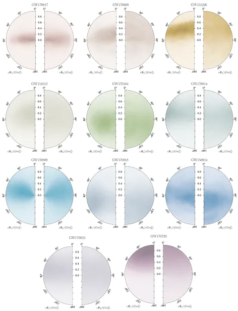
The remaining spin d.o.f. are due to a misalignment of the spin vectors with the normal to the orbital plane and give rise to a precession of the orbital plane and spin vectors around the total angular momentum of the binary. The bottom right in Fig. 5shows posterior and prior distribu-tions for the quantityχp, which encapsulates the dominant effective precession spin. The prior distribution for χp is induced by the spin prior assumptions (see AppendixesB 1 and C). Since χp and χeff are correlated, we show prior distributions conditioned on the χeff posteriors. The χp
posteriors are broad, covering the entire domain from 0 to 1, and are overall similar to the conditioned priors. A more detailed representation of the spin distributions is given in Fig.6, showing the probability of the spin magnitudes and tilt angles relative to the Newtonian orbital angular momentum. Deviations from uniformity in the shading indicate the strength of precession effects. Overall, it is easier to measure the spin of the heavier component in each binary [147,157]. None of the GW events exhibit clear precession. To quantify this result, we compute the Kullback-Leibler divergenceDKL[159]for the information gain from theχpprior to the posterior. Sinceχpandχeffare correlated, we can condition the prior on theχeff posterior
before we compute Dχp
KL. We give D
χp
KL values with and
without conditioning in TableVin AppendixB. Among the BBH events, the highest values of Dχp
KL are found for
GW170814 (0.13þ−00..0203 bits) and GW151226 (0.12þ−00..0205 bits). In all cases, the information gain for Dχp
KL is much
less than a single bit. Conversely, we gain more than one bit of information in χeff for several events (see Table Vand also TableVI). For very well measured quantities such as the chirp mass for GW170817, we can gain approximately 10 bits of information and come close to the information entropy [160] in the posterior data. A clear imprint of precession could also help break the degeneracy between the mass ratio and effective aligned spin [161–164]. We discuss the influence of the choice of priors for spin parameters (and distance) in AppendixC.
As a weighted average of the mass and aligned spin of the binary,χeffprovides a convenient tool to test models of
compact object binary spin properties via GW measurements [165–170]. Several authors suggest [171–179] how stellar binary evolutionary pathways leave imprints on the overall distribution of detected parameters such as masses and spins. By inferring the population properties of the events observed to date[55], we disfavor scenarios in which most black holes merge with large spins aligned with the binary’s orbital angular momentum. With more detections, it will be possible to determine, for example, if the BH spin is preferentially aligned or isotropically distributed.
For comparable-mass binaries, the spin of a remnant black hole comes predominantly from the orbital angular momentum of the progenitor binary at merger. For non-spinning equal-mass binaries, the final spin of the remnant is expected to be approximately 0.7 [180–184]. The final spin posteriors are more precisely constrained than the component spins and also the effective aligned spin χeff.
Masses and spins of the final black holes are shown in Fig. 4. Except for GW170729 with its sizable positive χeff ¼0.37þ−00..2521, the medians of all final spin distributions
are around approximately 0.7. The remnant of GW170729 has a median final spin ofaf¼0.81þ−00..1307and is consistent
with 0.7 at 90% confidence.
D. Distance, inclination, and sky location
The luminosity distancedLof a GW source is inversely proportional to the signal’s amplitude. Six BBH events (GW170104, GW170809, GW170818, GW151012, GW170823, and GW170729) have median distances of about a Gpc or beyond, the most distant of which is GW170729 at dL¼2840þ−13601400 Mpc, corresponding to a
redshift of0.49þ−00..2119. The closest BBH is GW170608, at
dL¼320þ−110120Mpc, while the BNS GW170817 is found at dL¼42þ−136 Mpc. The significant uncertainty in the
other hand, it has been pointed out that at LIGO’s and Virgo’s current sensitivities it is unlikely but not impossible that one of the GWs is multiply imaged. The analysis in Reference[190]concludes that lensing by massive galaxy clusters of one of our BBH GW detections can be rejected at the4σ level.
In the right in Fig.7, we show the joint posterior between the luminosity distance (or redshift) and source-frame chirp mass. We see that overall luminosity distance and chirp mass are positively correlated, as expected for unlensed BBHs observations.
An observed GW signal is registered with different arrival times at the detector sites. The observed time delays and amplitude and phase consistency of the signals at the sites allow us to localize the signal on the sky [191–193]. Two detectors can constrain the sky location to a broken annulus [194–197], and the presence of additional detectors in the network improves localization [19,198–200]. Figure 8 shows the sky localizations for all GW events. Both panels show posteriors in celestial coordinates which indicate the origin of the signal. In general, the credible regions of sky position are made up of a collection of disconnected components determined by the pattern of sensitivity of the individual detectors. The top shows localizations for confidently detectedO2events that were communicated to EM observers and are discussed further in Ref. [22]. The results for the credible regions and sky areas are different from those shown in Ref.[22]because of updates in the data calibration and choice of waveform models. The bottom shows localizations forO1events, along withO2events not previously released to EM observers. The sky area is expected to scale inversely with the square of the SNR [20,197]. This trend is followed for events detected by the two LIGO detectors. Several events (GW170729, GW170809, GW170814, GW170817, and GW170818) are observed with the two LIGO detectors and Virgo, which improves the sky localization[201]. The SNR contributed by Virgo can significantly shrink the area. We find the smallest 90% sky localization areas for GW170817: 16deg2 and GW170818: 39deg2.
parameters to vary independently rather than being deter-mined by a common equation of state [202]. Results are consistent with those presented previously in Ref.[97]with slight differences in the derived tidal deformability, dis-cussed below. Posterior distributions for SEOBNRv4T and TEOBResumS are obtained from RAPIDPE. In contrast to
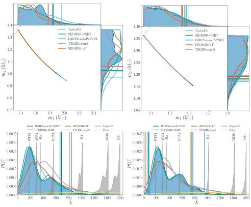
the BBH events discussed above, GW170817 is completely dominated by the inspiral phase of the binary coalescence. The merger and postmerger happen at frequencies above 1 kHz, where LIGO and Virgo are less sensitive. The distributions of component masses are shown in the top in Fig.9. With 90% probability, the mass of the larger NSm1
for the IMRPhenomPv2NRT model is contained in the range ½1.36;1.84M⊙ (½1.36;1.58 M⊙) and the smaller
NSm2 in ½1.03;1.36M⊙ (½1.18;1.36M⊙) for the
high-spin (low-high-spin) prior. In Fig.5, we show contours for the mass ratio and aligned effective spin posteriors for the IMRPhenomPv2NRT model assuming the high-spin prior. The results are consistent with those presented in Ref.[97]. The effective precession spinχpshown in the bottom right in Fig.5peaks at lower values than the prior, and the KL divergence Dχp
KL between this prior and the posterior is
0.19þ−00..0304bits. When conditioning the prior on the measured χeff,D
χp
KL decreases to 0.07þ−00..0201 bits, providing very little
evidence for precession. The strongly constrained χeff restricts most of the spin d.o.f. into the orbital plane, and in-plane spins are large only when the binary’s inclination angle approaches 180°, where they have the least impact on the waveform.
very close, 664, and the value for TaylorF2 is higher at 816. For SEOBNRv4T and TEOBResumS, we find 843 and 841, respectively. For the low-spin prior, we quote the two-sided 90% highest posterior density (HPD) credible interval onΛ˜ that does not containΛ˜ ¼0. This 90% HPD interval is the smallest interval that contains 90% of the probability. For IMRPhenomPv2NRT, we obtain Λ˜ ¼330þ−251438, which is slightly higher than the interval 300þ−230420 found in Ref. [97]. For SEOBNRv4NRT, we find Λ˜ ¼305þ−241432 and for TaylorF2 394þ−321557. For SEOBNRv4T and TEOBResumS, we find349þ−349394and405þ−375545, respectively. The posteriors produced by these two models agree better for the low-spin prior. This result is consistent with the very good agreement between the models for small spinsjχij≤ 0.15 shown in Ref. [33]. For reference, we also show contours for a representative subset of theoretical EOS models given by piecewise-polytrope fits from Ref.[203]. These fits are evaluated using the IMRPhenomPv2NRT component mass posteriors, and the sharp cutoff to the right of each EOS posterior corresponds to the equal mass ratio boundary. As found in Ref.[97], the EOSs MS1, MS1b, and H4 lie outside the 90% credible upper limit and are therefore disfavored.
In TableIII, we quote conservative estimates of key final-state parameters for GW170817 obtained from fits to NR simulations of quasicircular binary neutron star mergers [204–206]. We do not assume the type of final remnant and quote quantities at either the moment of merger or after the postmerger GW transient. Lower limits of radiated energy up to the merger and peak luminosity are given at 1% credible level. The final mass is computed from the radiated energy including the postmerger transient as an upper limit at 99% credible level. For the final angular momentum, we quote an upper bound computed from the radiated energy and using the phenomenological universal relation found in Ref. [204].
F. Comparison against previously published results We compare PE results between the original published
O1 and O2 analyses for GW150914, GW151012, GW151226, GW170104, GW170608, and GW170814 and the reanalysis performed here. The values presented here supersede previously published results. For some events, we see differences in the overall posteriors that are due to a different choice of waveform models that have been combined. This difference is especially the case when comparing against previous results that combine samples between spin-aligned and effective precession models and mostly affects spin parameters. We first mention differences that are apparent when comparing results from the same waveform models in the original analysis and the reanalysis.
The source-frame total mass is consistent with the original analysis. For GW150914, we find an increase in
the median of about1M⊙in this reanalysis when
compar-ing between the same precesscompar-ing waveform models because of the improved method for computing the power spectral density of the detector noise and the use of frequency-dependent calibration envelopes. For GW170104, we find the median of the total mass to be0.3M⊙higher because of
the recalibration of the data and the noise subtraction. Similarly, we find an increase of about0.2M⊙ in the total
mass for GW151012 and a decrease in the total mass of about0.3M⊙for GW151226 and0.2 M⊙for GW170608
in the reanalysis. The mass ratio and effective spin parameters are broadly consistent with the original analysis. GW170104 especially benefits from the noise subtraction. This subtraction increases the matched-filter SNR recovered by the parameter-estimation analysis from 13.3þ−00..32to14.0þ−00..32. The increase in SNR results in reduced parameter uncertainties[128]. For the effective spin param-eter, the tightening of the posterior results in the loss of the tail at low values. The inferred value changes from −0.12þ−00..3021 to −0.04þ−00..2117; the upper limit remains about the same, and there is still little support for large aligned spins. For GW151226, we find from using the fully precessing model that the inferred effective aligned spin is 0.15þ−00..1125, and with the effective precession model it is 0.20þ−00..0818. The fully precessing model has some support at χeff ¼0; the probability thatχeff<0is, however,<0.01. We
find with 99% probability that at least one spin magnitude is greater than 0.28 compared to the value 0.2 in theO1
analysis. We discuss further differences between results obtained from the two BBH waveform models in AppendixB 2.
VI. WAVEFORM RECONSTRUCTIONS
In the previous section, we present estimates of the source properties for each event based on different rela-tivistic models of the emitted gravitational waveform. Such models, however, do not necessarily incorporate all physi-cal effects. Here, we take an independent approach to determine the GW signal present in the data and assess the consistency with the waveform model-based analysis.
Figure10shows the time-frequency maps of the gravi-tational-wave strain data measured in the detector where the higher SNR is recorded[207], as well as three different types of waveform reconstructions for all GW events from BBHs. Two of those waveform reconstructions provide an independent estimate of the most probable signal: Instead of relying on waveform models, these algorithms exclu-sively use the coherent gravitational-wave energy measured by the detector network, requiring only weak assumptions on the form of the signal for the reconstruction.
The first method, BAYESWAVE, represents the waveform
as a sum of sine-Gaussian waveletshðλ;⃗ tÞ ¼Pj¼N1Ψðλj;⃗ tÞ,
where the number of wavelets used in the reconstruction,