Data Computational Modelling of Multivariable
Non-Stationary Noisy Linear Systems by
MOESP_AOKI_VAR Algorithm
Johanna B. Tobar and Celso P. Bottura
Abstract—The main objective of this work is to develop
a recursive algorithm for identification in the state-space of linear stochastic discrete multivariable non-stationary system; a computational process called MOESP_AOKI_VAR is proposed and implemented to achieve this. The proposed algorithm is based on the subspace methods: Multivariable Output-Error State Space (MOESP), used for computational modelling of systems and on an AOKI algorithm developed by Masanao Aoki, for computational modelling of time series that we call the Aoki algorithm.
Index Terms—MOESP, Markov parameters, non-stationary system, time series, identification, Aoki.
I. INTRODUCTION
A
n initial study of different kind of systems for iden-tification, based on the state-space, is performed. Ad-ditionally, a structure to be used in the problem resolution of computational modelling for non-stationary noisy linear systems is proposed. Through this study, non-stationary sys-tems are treated as a group of invariant models with respect to the time. It is also considered that the matrix systemAK, BK, CK, DK,presents small changes with respect to the time. This is translated into continuous and slow changes within the matrices and it allows for the generation of a recursive algorithm, which is the main objective of this study. A linear system is considered as the superposition of its deterministic and stochastic part. A MOESP_VAR algorithm is used for modelling the deterministic part, whilst the stochastic part is modelled by the use of AOKI_VAR algorithm. Finally, the algorithm is tested by using a benchmark.
II. FOUNDATION
A. Stationary Deterministic Linear System
The representation of the deterministic linear system in state spaces has the following form:
xk+1=Axk+Buk
yk =Cxk+Duk (1)
where, xk ∈ Rn is the state vector, uk ∈Rm is the input vector and yk ∈Rl is the output vector. TheA, B, C andD matrices are considered constant for everyk instant.
Johanna Tobar is with the Department of Energy Sciences and Mechanics, University of the Armed Forces, Quito, Ecuador, e-mail: Celso Bottura is with the Department of Machines, components and intelligent systems, State University of Campinas, Campinas, Brasil, e-mail:
B. Stationary Noisy Linear System
In order to quantify the uncertainty and external perturba-tions of the system, vk and wk are added in the state-space equations. These terms are considered as inputs where non-control exists:
xk+1=Axk+vk
yk =Cxk+wk (2)
The pertubation vectors vk ∈ Rn and wk ∈ Rl are random variables with zero means. The sequences
(vk, k= 0,±1,±2, ...) and (wk, k= 0,±1,±2, ...) are considered stochastic processes of Gaussian white noise. Additionally, the stochastic process can be represented by
defining the error vector as ek =
wk
vk
, with E[ek] =
0 ∀k, and its innovation representation is the following:
xk+1=Axk+Kek
yk=Cxk+ek (3)
where,ek is a white noise sequence and its covariance matrix is given by∆ =E ekeTk
.
When referring to the covariance domain, the Markov parameters of the system can be represented as:
Λi=
CΠ0CT +R i= 0
GT AT−i−1
CT i <0
CAi−1G i≥1
(4)
where, Gis also presented as G=AΠ0CT +S, yielding as result the following:
R= Λ0−CP CT
Q=P−AP AT
S=M−AP CT
(5)
The stochastic realization problem consists of finding one or more models in the state-space through process statistical data such us covariance. For further information read Caceres, Angel Fernando Torrico (2005), Tamariz, Annabell (2005) and Barreto, G. (2002).
C. Non-stationary Deterministic Linear System.
A non-stationary deterministic linear system is represented by the following state-space equations:
xj,k+1=Aj,kxj,k+Bj,kuj,k
being j ∈[j0, j0+n−1] and k ∈ [k0, k0+T−1] , where
j0 is the first interval of experiment,k0 is the first instant of the experiment, n is the total number of simple experiments andT ≥n. Equation (6) can also be expressed as:
yH=OkXH+TkUH (7)
To get detailed information about the process to obtain the equation (7), consult the matricesyH,Ok,XH,TkyUH on [2].
D. Non-stationary Noisy Linear System
A non-stationary noisy linear system is expressed as
fol-lows:
xj,k+1=Aj,kxj,k+Bj,kuj,k+vj,k
yj,k=Cj,kxj,k+Dj,kuj,k+wj,k (8)
being j ∈[j0, j0+n−1] and k ∈ [k0, k0+T−1] , where
j0is the first interval of the experiment,k0 is the first instant of time of the experiment, n is the total number of simple experiments, T ≥ n and vj,k ∈ Rn and wj,k ∈ Rl are random variables of null arithmetic mean, and the sequences
(vk, k= 0,±1,±2, ...) and (wk, k= 0,±1,±2, ...) are non-stationary stochastic processes that are generated by the non-stationary stochastic system represented by the state-space equation:
xj,k+1=Aj,kxj,k+Kj,kej,k
yj,k=Cj,kxj,k+ej,k (9)
where, ek is the white noise stochastic process.
E. Time Variant Identification
The identification algorithm works on the assumption that time-varying systems can be treated as a set of time-invariant models for a given time interval. Thus, the identification of time-varying systems consists of a set of n time-invariant models which describes the system for the defined experiment. The following expression relates the input variables to the state vector in a time variant linear system in thekthmoment:
xk =A(k−1)x0+ k−1 X l=0
A(k−l−1)Blul (10)
where, A(n)andA(n)represent the transition matrixes that satisfy:
A(0)=A0
A(0)=I
A(n)=AnA(n−1)=An. . . A2A1A0
A(n)=A
nA(n−1)=An. . . A2A1
(11)
A set of indices are stated to interpret the identification of problem parameters; additionally, the set of indicesj, konuj,k indicates the sample input for instant kth and for system ex-perimentation range jth(8). Furthermore,j∈[j
0,j0+n−1] and k ∈ [k0,k0+T−1], where j0 is the first range of experimentation, k0 is the first instant of time, n is the total number of experiments or tests andT is the time required for a single experiment.
The problem to be solved is represented by the state-space model:
xj,k+1
yj,k
=
Ak Bk
Ck Dk
xj,k
uj,k
(12)
based on the following output data sequence:
Yj,k=
yj0,k0 yj0,k0+1 · · · yj0,k0+T−1 yj0+1,k0 yj0+1,k0+1 · · · yj0+1,k0+T−1
..
. ... · · · ...
yj0+n−1,k0 yj0+n−1,k0+1 · · · yj0+n−1,k0+T−1
(13) The problem is also based on the input sequenceUj,k for the same series of experiments and same time interval. The matrix
Yj,krepresents the set of(n−1)intervals of experimentation. It allows to develop general expressions that govern the system and it also relates the inputs and outputs at a start timek0and establishes a correct experimentation intervalj, for a discrete time variant system, which is represented in state space by:
xj,k+1=Akxj,k+Bkuj,k
yj,k=Ckxj,k+Dkuj,k (14)
for the next instant, the expression is:
xj,k+2 =Ak+1xj,k+1+Bk+1uj,k+1
yj,k+1=Ck+1xj,k+1+Dk+1uj,k+1 (15)
plugging in equation (15) into equation (14) yields:
xj,k+2=Ak+1Akxj,k+Ak+1Bkuj,k+Bk+1uj,k+1
yyj,k+1=Ck+1Akxj,k+Ck+1Bkuj,k+Dk+1uj,k+1 (16) and this process is repeated successively. Solving equation (14) for any moment of time k0 ≥ 0, the solution can be written as:
yj,l=
Cl,j+Dluj,l + l= 0
ClA(l−1)xj,l+
+ l−1 X i=0
ClA(l−i−1)Biuj,i+Dluj,l l > k0 (17)
Equation (14) can be rewritten in a shorter form by the extended model:
YH=OkXH+TkUH (18)
1) Determination of the extended model: For an experiment
j, the matrix UH for the stationary case is equal to the matrix UH from the time-varying case. Data from a single experiment is assumed. To solve the non-stationary discrete case is necessary to assume that data is available from a single experiment.
QR Factorization Update:
a.- Let’s assume that the following measurements were already processed by the algorithm:
[uj0,k0 uj0,k0+1 ... uj0,k0+T−1]T and
[yj0,k0 yj0,k0+1 ... yj0,k0+T−1]T b.- Being the QR factorization:
Rj0,11 0
Rj0,21 Rj0,22
Qj0,1
Qj0,2
(19)
where,j0 represents the set of input-output values pro-cessed in the most recent experiment.
c.- Finally, suppose that during the time interval
[j0, j0+n−1] the model in state space is invariant and equal to:
xk+1=Aj0xk+Bj0uk
yk=Cj0xk+Dj0uk (20)
It can also be represented in a shorter form by relating the different data matrices as:
YH=OkXH+Tj0,kUH (21)
3) Recursive algorithm for the stochastic part: See [2] : F. State-Space Deterministic-Stochastic Modelling of the Non-stationary System
One way of representing non-stationary discrete multivariate noisy linear systems, with exogenous time variable inputs in the state space is:
xj,k+1=Aj,kxj,k+Bj,kuj,k+vj,k
yj,k=Cj,kxj,k+Dj,kuj,k+wj,k (22)
with
E
vj,k
wj,k
vT j,s wTj,s
=
Q S
ST R
k=s
0 k6=s
(23) A theorem for the decomposition by superposition of noisy time variant linear systems is proposed as follows:
Theorem 1. By superposition, a variant time noisy linear modelS,in an innovative form given by:
S:
xj,k+1=Aj,kxj,k+Bj,kuj,k+Kj,kej,k
yj,k=Cj,kxj,k+Dj,kuj,k+ej,k (24)
can be decomposed into the following two subsystems:
Sd:
xd
j,k+1=Aj,kxdj,k+Bj,kuj,k
yd
j,k=Cj,kxdj,k+Dj,kuj,k (25) and
Se: xe
j,k+1=Aj,kxej,k+Kj,kej,k
ye
j,k=Cj,kxej,k+ej,k (26) where, the superscriptsd anderefer to the determistic and the stochastic subsystems Sd andSe respectively andyj,k=
yd
j,k+yj,ke . The noisy signal state is:xj,k=
xd j,k
xe j,k
where,
A=
Ad 0 0 Ae
B =
Bd 0
C=
Cd Ce
D=Dd, K=Ke
Proof: See [1]
III. MOESP_AOKI_VAR ALGORITHM
The proposed algorithm MOESP_AOKI_VAR collects the MOESP_VAR proposed in [2], [3] and the MOESP_AOKI proposed in [1], [2] and the AOKI_VAR in [13], [14] re-spectively. Therefore, the algorithm MOESP_AOKI_VAR is as follows:
1) Obtain the Hankel matricesYH andUH 2) Perform the QR factorization:
UH
YH
=
R11 0
R21 R22
Q1
Q2
(27)
where, R11 andR22 are invertible square matrices. 3) Compute the SVD ofR22 as:
R22= UH UH⊥
P
n 0
0 P
2
VT n (Vn)T
(28)
4) Solve the equation system:
UH(1)AT =UH(2) (29)
5) Update: The recursive algorithm shown in section II.E.2 is applied
Thus, obtaining the matrices Ad
j,k, Bj,kd , Cj,kd , Dj,kd , of
yd
j,kfor eachktime instant andj intervals with respect to the time.
6) Determine the signal generated by the matrices
HA, HM, HC, H, Y −, Y+
Y−=
¯
y1 y¯2 y¯3 · · · yN¯−1 0 y¯1 y¯2 · · · yN¯−2 0 0 y¯1 · · · yN¯−3
..
. ... ... · · · ...
0 0 . . . yN−¯k−1 yN¯−k
Y+=
¯
y2 y¯3 y¯4 · · · y¯N ¯
y3 y¯4 y¯5 · · · 0 ¯
y4 y¯5 y¯6 · · · 0 ..
. ... ... · · · ...
¯
yj+1 yj+2¯ yj+3¯ · · · 0
H = Y+Y T
−
N =
Λ1 Λ2 · · · Λk Λ2 Λ3 · · · Λk+1
..
. ... . .. ...
HA=
Λ2 Λ3 · · · Λk+1 Λ3 Λ4 · · · Λk+2
..
. ... . .. ...
Λj+1 Λj+2 · · · Λj+k+1
HM =
Λ1 Λ2 .. .
Λj
HC=
Λ1 Λ2 · · · Λk
7) Obtain the SVD for the covariance Hankel matrix
H =UP1/2P1/2 VT
8) Calculate the matrices Ae
j,k, Cj,ke , Kj,ke 9) Validate.
IV. EXPERIMENTATION AND RESULTS
The proposed algorithm is initially defined for T intervals of experimentation thus getting the system matrices identifica-tion. The presented MOESP_AOKI_VAR is assessed T times in order to determine T sets of matrices corresponding to each experiment.
If ∇ represents small increments, Lj is an integer number for each Ij experimentation interval stated by:
Ij= [kj−Lj∇, kj+Lj∇] (30)
to validate the proposed algorithm a benchmark is imple-mented [4]. The identification at time instant kj (which is the middle point of each interval Ij) is determined as
kj+1=kj+v∇, where v is an integer number,∇represents an increment with respect to the simulation time and it is given by ∇=M∇j, where ∇j is thej−thsampling period and
M is an integer number.Lj = 500∀jis defined for this study. The benchmark system is:
The deterministic part is given by the following matrices
Ak=
−0.3 ak 1 −1
(31)
where,
ak=− 1 3−
1 10sen(
2πk
400)
and the remaining matrices are consired constants:
Bk=
−2 1
1 1
; Ck =
1 3 1 2
(32)
Dk= 0
The system input is randomically changing for each iteration of the algorithm.
The proposed algorithm presents the following results for
k= 1:
Aj,k=
−0.3000 0 0 −0.4040
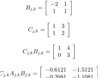
Bj,k=
−2 1 1 1
Cj,k=
1 3 1 2
Cj,kBj,k=
1 4 0 3
Cj,kAj,kBj,k=
−0.6121 −1.5121
−0.2081 −1.1081
The deterministic-stochastic identification of the system under noise is realized. The obtained results after running the first part of the algorithm MOESP_AOKI_VAR are shown:
Adj,k=
−0.3000 0
−0.0000 −0.4077
Bj,kd =
4.1559 3.7636
−3.1924 1.5997
Cj,kd =
0.7705 0.6867 0.5137 0.6677
Cj,kd Bj,kd =
1.0098 3.9984 0.0031 3.0014
Cj,kd Adj,kBj,kd =
−0.6478 −1.5118
[image:4.612.355.519.51.182.2]−0.2308 −1.1086
[image:4.612.102.270.51.185.2]Figure 1 shows the output of the deterministic model
Figure 1. Output of the deterministic subsystem
The results after running the second part of the algorithm MOESP_AOKI_VAR are:
∆ = [1.6092]
Aej,k=
−0.2092 −0.7319 0.7319 0.1218
Kj,k=
−0.2582 1.1257
Cj,ke =
where, ∆ is the covariance matrix of the noise.
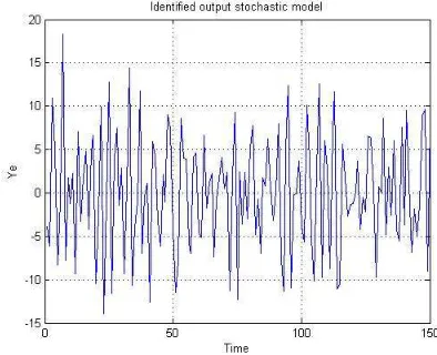
Figure 2 presents the stochastic modeled signal by using the second part of the algorithm MOESP_AOKI_VAR
Figure 2. Output of the stochastic subsystem
Figure 3 displays the overlapped signals of the deterministic and stochastic output signals yd
j,k andyj,ke .
Finally, a verification and validation process of the proposed combined algorithm MOESP_AOKI_VARis performed and Figure 4 shows the results.
[image:5.612.70.268.382.725.2]The algorithm MOESP_AOKI_VAR describes satisfacto-rily the noisy signals.
Figure 3. Overlapping signals
Figure 4. Error
V. CONCLUSIONS
A computational procedure is formulated for the identifi-cation of discrete stochastic multivariate linear systems time variant. The considered hypothesis is that the variation in time of the dynamic system is sufficiently slow to guar-antee the efficiency of the subspace identification MOESP for a non-stationary noisy linear system. The algorithm MOESP_AOKI_VAR has its foundation in AOKI and MOESP algorithms and it is given by the superposition of them. The obtained results describe that the proposed method guarantee an apropriate behaviour when modeling this kind of systems.
REFERENCES
[1] Aoki, Masanao, “State Space Modeling of Time Series”, Springer Verlag, 1987.
[2] Cáceres, Angel Fernando Torrico, "Identificação e Controle Estocásticos Decentralizados de Sistemas Interconectados Multivariáveis no Espaço de Estado", PhD Thesis, FEEC-UNICAMP, 2005.
[3] Tamariz, A.D.R., "Modelagem Computacional de Dados e Controle Inteligente no Espaço de Estados". PhD Thesis, LCSI/FEEC/UNICAMP, Campinas SP, Brasil, 2005.
[4] Tamariz A.D.R., Bottura C.P., Barreto G., "Iterative MOESP Type Algorithm for Discrete Time Variant System Identification", Proceedings of the 13th Mediterranean Conference on Control and Automation, (MED’2005), Limassol, Cyprus, June 27-29, 2005.
[5] Ohsumi, Akira and Kawano T., "Subspace Identification for a Class of Time-Varying Continuous-Time Stochastic Systems Via Distribution Based Approach”, Proceedings 15th IFAC World Congress, Barcelona, July 2002.
[6] Barreto, G., "Modelagem Computacional Distribuída e Paralela de Sistemas e de Séries Temporais Multivariáveis no Espaço de Estado”, PhD Thesis, FEEC-UNICAMP, 2002.
[7] Dewilde, Patrick and Van der Veen, Alle-Jan, "Time-Varying Systems and Computations", Kluwer Academic Publishers, 1998.
[8] Shokoohi, S. and Silverman, L.M., "Identification and Model Reduction of Time-Varying Discrete-Time Systems", Automatica 23, pp. 509-522, 1987.
[9] Tamariz A.D.R., Bottura C.P. and Barreto G., “Algoritmo Iterativo do tipo MOESP para Identificação de sistemas discretos variantes no tempo - Parte I: Formulação”, DINCON, 2003.
[10] Tamariz A.D.R., Bottura C.P. and Barreto G., “Algoritmo Iterativo do tipo MOESP para Identificação de sistemas discretos variantes no tempo - Parte II: Implementação e Experimentação”, DINCON, 2003. [11] Tamariz A.D.R. and Bottura C.P,“Proposta para Identifacação de
sis-temas ruidosos multivariaveis no espaço de estado”, DINCON, 2007. [12] Verhaegen, Michel and Deprettere, E., “A fast recursive MIMO State
Space model Identification Algorithm”, Proceedings of the 30th Con-ference on Decision and Control, Brighton, England, December 1991. [13] Verhaegen, Michel and Dewilde, Patrick., “Subspace Model
Identifica-tion - Part 1 : The outputerror state-space model identificaIdentifica-tion class of algorithms”, International Journal of Control, Volume 56, Number 5, 1187-1210, November, 1992.
[14] Verhaegen, Michel and Yu Xiaode, "A Class of Subspace Model Identification Algorithms to Identify Periodically and Arbitrarily Time-varying Systems", Automatica, Vol. 31, N0. 2, pp. 201-216, 1995. [15] Tobar Johanna, Bottura Celso and Giesbrechtr Mateus, "Computational
Modeling of Multivariable Non-Stationary Time Series in the State Space by the AOKI_VAR Algorithm", IAENG International Journal of Computer Science, 2010.