Online Full Text



Abstract—We applied traditional time series analysis and artificial neural network (ANN) techniques to model and forecast the power consumption of Bangkok’s metropolitan area. Time series data in terms of units of household electricity usage were obtained from the Metropolitan Electricity Authority of Thailand. The data had been collected monthly from January 2010 to May 2015. Forecasting models with different parameters are generated from both techniques using the training data, which are the series from January 2010 to December 2014. The remaining data from January 2015 to May 2015 are employed as the testing data. Forecasting performance of each model is measured by the rooted mean square error (RMSE) and the mean absolute percentage error (MAPE) metrics. The traditional time series forecasting models studied in this research are GLM, HoltWinters, and ARIMA. For ANN, we examine four models using 3 layers with different number of neurons ranging from 4 to 7: 3L-4N,3L-5N, 3L-6N, and 3L-7N. The experimental results reveal that ARIMA is superior among the traditional time series models. For the intelligent based models, 3L-6N is the best of ANN models. Moreover, the MAPE metric of the 3L-6N model is less than the ARIMA model. As a result, we can conclude that ANN model is more powerful in forecasting power distribution units than the traditional time series models.

Index Terms—Artificial neural networks, forecasting, time series model, electrical load analysis

I. INTRODUCTION

HIS research aims to perform time series analysis to forecast future data by using electricity supply information of Metropolitan Electricity Authority of Thailand. It is a monthly reported data from January 2010 to May 2015. The data are presented in unit metric in which 1 unit refers to 1000 kilowatts per hour. These data contain the time series pattern.

Manuscript December 26, 2015; revised January 18, 2016. This work has been supported in part by grants from Suranaree University of Technology through the funding of the Data Engineering Research Unit.

R. Chuentawat is a doctoral student with the School of Computer Engineering, Suranaree University of Technology, and also an assistant professor at Nakhon Ratchasima Rajabhat University, Nakhon Ratchasima 30000, Thailand (e-mail: [email protected]).

S. Bunrit is a doctoral student with the School of Computer Engineering, Suranaree University of Technology, Nakhon Ratchasima 30000, Thailand (e-mail: [email protected]).

C. Ruangudomsakul is a doctoral student with the School of Computer Engineering, Suranaree University of Technology, and also a lecturer at Sisaket Rajabhat University, Thailand (e-mail: [email protected]).

N. Kerdprasop is an associate professor with the School of Computer Engineering, Suranaree University of Technology, Nakhon Ratchasima 30000, Thailand (e-mail: [email protected]).

K. Kerdprasop is an associate professor with the School of Computer Engineering, Suranaree University of Technology, Nakhon Ratchasima 30000, Thailand (e-mail: [email protected]).

An accurate forecast on the demand of electricity provides the advantageous information in resource planning,management of funding, and reducing the operation cost. Bunn and Farmer [2] found and reported that 1% of forecasting error raised by 10 million units of the operation costs. Therefore, the precision of forecast is a challenging problem, especially on the demand of electricity supply.

Traditional time series forecasting technique generates the forecasting model from the training data set by determining the unrecognized parameters. In our study, simple linear regression analysis, triple exponential smoothing and autoregressive integrated moving average (ARIMA) of Box and Jenkins method are applied. The acquired forecasting models from the three methods are then compared the accuracy using the two metrics: rooted mean square error (RMSE) and mean absolute percentage error (MAPE). The lower RMSE and MAPE, the more accurate the model is.

Artificial neural network (ANN) is a machine learning technique that mimics the concept of neuron operation in human brain. It can be used to forecast time series data by setting the output neuron to provide the observed value at time t (yt ). Input is the observed value of lag time from 1 to p period prior to the time t (yt-1, yt-2, …, yt-p). In this study, we used three-layer feed-forward back propagation neural network for time series analysis. We compared each model to find the most suitable one with the lowest RMSE and MAPE.

Our research is thus a comparative study of artificial neural networks and traditional time series analysis for forecasting time series data. Research objectives are:

1.Apply three traditional time series analysis methods for generating forecasting model using the R language. Such methods are generalized linear models (GLM), Holt-Winters (HoltWinters) and autoregressive integrated moving average (ARIMA).

2.Apply ANN models for time series analysis by generating forecasting models in Matlab.

3.Find the most suitable forecasting model by comparing RMSE and MAPE resulting from all traditional time series analysis methods and ANN models.

II. LITERATURE REVIEW

There are a number of related works in literatures about time series analysis using traditional time series methods and ANNs.

Maçaira, Souza and Oliveira [3] studied about how to define forecasting model and forecast yearly electricity consumption of residential units in Brazil until 2050 using

Artificial Neural Networks and Time Series

Models for Electrical Load Analysis

Ronnachai Chuentawat*, Supaporn Bunrit, Chanintorn Ruangudomsakul, Nittaya Kerdprasop, and

Kittisak Kerdprasop

Pegels exponential smoothing forecasting technique. They performed parameter adjustment for forecasting data along with the estimated value that is available in PDE (the ten year energy planning) and PNE (the nation energy planning). The result was that the Pegels exponential smoothing forecasting technique produced the nearest estimation of electrical consumption in both PDE and PNE.

Keka and Hamiti [4] did experiment to find mathematical model representing relationship between electrical energyand time by using linear regression techniques. They used electrical supply data collected from the electrical substation every 15 minutes and set the time interval by using day, week and month. Result from the experiment showed a linear mathematical model that can represent the relationship between electrical energyand time.

Chujai, Kerdprasop and Kerdprasop [5] studied time-series analysis of household electrical consumption using data from UCI Machine Learning Repository. They generated forecast models from ARIMA and ARMA using 4 kinds of time interval (day, week, month, and quarter) and experimented with the R language. They performed model tolerant analysis by measuring the AIC (Akaike Information Criterion) and RMSE. The result showed that the ARIMA model is suitable for forecasting data in the month and quarter interval while the ARMA model is suitable for forecasting data in day and week interval.

Wang and Ming [6] studied about forecasting energy consumption in China using ARIMA, ANN and hybrid ARIMA-ANN model. They compared the accuracy using RMSE, MAE (Mean Absolute Error), and MAPE. The result of the study showed that a hybrid model provided better accuracy in forecasting than either the ARIMA, or ANNs.

Firata, Turanb and Yurdusev [7] studied about forecasting water supply consumption in Turkey using several ANN techniques including generalized regression neural networks (GRNN), cascade correlation neural network (CCNN), and feed forward neural networks (FFNN). They defined 6 network structures and then performed statistical testing by measuring the average absolute relative error (AARE), normalized root mean square error (NRMSE), and threshold statistic (Ts). The result showed that the values of AAER and NRMSE of the M5 models are better than those of the other modelsand the test statistics of the M5 CCNN model is slightly better than those of GRNN and FFNN models.

III. METHODOLOGY A. Traditional Time Series Models

In traditional time series forecasting technique, we apply general linear regression, triple exponential smoothing, and Box and Jenkins methods. We then forecast data for the next 5 intervals. After that, we compare forecasted data against real data in a test set. The RMSE and MAPE metrics are used as statistical measure instruments to find the suitable forecasting model. The 3 traditional forecasting techniques (GLM, HoltWinters, and ARIMA) are described as follows:

1. GLM model is the forecasting model that are generated by simple linear regression analysis. GLM linear regression [8] is as shown in equation 1.

Y = 0 + 1X +  (1)

where X is a time-interval variable in a monthly unit, Y is the amount of monthly power distribution unit,

 is a residual term.

2. HoltWinters model is deriving from triple exponential smoothing. It is a smoothing technique that can be used to generate forecast models from data with trend and seasonal [9]. HoltWinters model can be described as in equations 2-4. To forecast the future event, equation 5 which is composed of the level, trend, and seasonal parts is applied.

Level : (2)

Trend : (3)

Seasonal : (4)

Forecast : (5)

where α is constant for level smoothing β is constant for trend smoothing γ is constant for seasonal smoothing Lt isestimated level of time series attime t Yt is observed value at time t

bt isestimated slopeof time series attime t St is seasonal factor

s is seasonal length, equal to 12 months (s = 12) m is forecast intervals

Ft+m is forecasted value m intervals

3. ARIMA model is a model derived from Box and Jenkins method. General term of ARIMA [10] can be presented with backward shift operator (B) as in equation 6.

(6) where and

In order to generate an ARIMA model, we have to analyze time series data for defining suitable parameters of ARIMA(p, d, q)x(P, D, Q)S. That means selecting the suitable p, d, q from trend and P,D,Q from seasonal. In R language, we can use function auto.arima() to assign suitable ARIMA(p, d, q)x(P, D, Q)S. In this research, we use (p, d, q) = (1, 0, 0) and (P, D, Q)S = (1, 0, 0)12 , where 1 season = 12 months (S=12). Therefore, a suitable ARIMA(p, d, q)x(P, D, Q)S is ARIMA(1, 0, 0)x(1, 0, 0)12.

After obtaining 3 forecasting models from the 3 methods mentioned above, statistical measuring in terms of RMSE and MAPE is compared for model accuracy. A model with the lowest RMSE and MAPE is the most suitable one. Summary of steps in applying traditional time series analysis to find a suitable forecasting model is shown in figure 1.

Fig.1. Steps in selecting the most appropriated model for forecasting time series data

Fig. 2. Time series data are created from secondary data

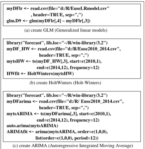
Fig. 3. R commands for generating traditional forecasting model

Step 2: Transform data to be time series. The data from the monthly report of the Metropolitan Electricity Authority is a monthly interval from January 2010 to May 2015 as shown in figure 2. We divide the data into 2 sets. The first is a training set consisting of data from January 2010 to December 2014. It is used for generating the forecasting model. The test set is data from January 2015 to May 2015. Test data are used for validating the model and evaluating by RMSE and MAPE.

Step 3: Model time series data. This step generates 3 different forecasting models from the training set. We build 3 forecasting models from the same training set with commands in R language that can be summarized in figure 3.

Step 4: Compare models with statistical measurements RMSE and MAPE. The computation of RMSE (rooted mean square error) and MAPE (mean absolute percentage error) [11] is shown in equations 7 and 8, respectively.

RMSE = (7)

MAPE = (8)

where yt is observed value at time t, ŷt is forecasted value at time t, and n is the number of forecasting period.

Step 5: Report the best model. The bestforecasting model is the one with the lowest RMSE and MAPE values.

B. Artificial Neural Network Model

Artificial neural networks (ANNs) are the simulated networks of neurons in the human brain. We can apply ANNs to forecast time series data. ANNs perform learning from existing data by analyzing the correlation between observed values at current time with previous observed values. After getting an ANN model from the training set, we can use such model to forecast the value of new observation in the test set.

In this research, we use ANNs model calls three-layer feed-forward back propagation neural networks which has 1 hidden layer. Output from a model is a forecasting value at current time (yt). Input to a model is the previous observed values at 1 to p time intervals (yt-1, yt-2, …, yt-p) and be represented as a vector. The correlation between input and output [6] can be shown as in equation 9.

(9) where (j=1,…,q) and (i=0,…,p; j=1,…,q) are

model parameters which are called weights , p is the number of neurons in the input layer, q is the number of neurons in the hidden layer and

have sigmoid function [6] as a transfer function presented in equation 10.

From ANNs model shown in equation 9, we can transform to nonlinear function to represent the relationship [6] between previous observed values (yt-1, yt-2, …, yt-p) and forecasting value (yt) as in equation 11.

(11) where is a vector of all parameters andf is a function used for determining the network structure and the connecting of weights. As a result, the neural network model is equivalent to and can be expressed in terms of nonlinear autoregressive model.

In the research on Wang and Meng [6], they suggested that ARIMA and ANNs have something similar. From our ARIMA model, it has p = 1 and P = 1 which means observation at time t (yt) relates to the previous observation with a lag of one interval (yt-1) and relates to previous observation with 1 season lag or 12 Collect data from secondary source

(The report of electricity supply situation)

Transform data to be time series

Model time series data

GLM model HoltWinters model ARIMA model

Compare models with statistical measurement RMSE and MAPE

Report the best model

myDFlr <- read.csv(file="d:/R/EuseLRmodel.csv" , header=TRUE, sep=",")

glm.D9 <- glm(myDFlr[,4] ~ myDFlr[,3])

(a) create GLM (Generalized linear models)

library("forecast", lib.loc="~/R/win-library/3.2") myDF_HW <- read.csv(file="d:/R/Euse2010_2014.csv", header=TRUE, sep=",")

mytsHW <- ts(myDF_HW[,3], start=c(2010,1),

end=c(2014,12), frequency=12)

HWfit <-HoltWinters(mytsHW)

(b) create HoltWinters (Holt-Winters)

library("forecast", lib.loc="~/R/win-library/3.2") myDFarima <- read.csv(file="d:/R/Euse2010_2014.csv", header=TRUE, sep=",")

mytsARIMA <- ts(myDFarima[,3], start=c(2010,1),

end=c(2014,12), frequency=12) auto.arima(mytsARIMA)

ARIMAfit <- arima(mytsARIMA, order=c(1,0,0),

list(order=c(1,0,0), period=12))

intervals (yt-12). So, we can use yt-1 and yt-12 as the input to ANNs model. Therefore, input layer of ANNs model has 2 neurons. In order to investigate the complexity of an ANN causing the over-fitting problem, we experiment with 4 ANNs models defined as follows:

Model 1: Three layers, two input neurons, one hidden neuron and one output neuron (3L-4N). Model 2: Three layers, two input neurons, two hidden

neurons and one output neuron (3L-5N). Model 3: Three layers, two input neurons, three hidden

neurons and one output neuron (3L-6N). Model 4: Three layers, two input neurons, four hidden

neurons and one output neuron (3L-7N).

Fig. 4. Examples of data file for generating ANNs model

Fig. 5. Command sets in Matlab for generating ANNs model

We then implement our ANNs structures using Matlab software and the steps can be described as follows:

Step 1. Create 3 data files with Excel (figure 4) for generating models. The first file is AllEuse; it contains a power distribution unit data from January 2010 to May 2015. The second file is InputTraining; it contains a training set as input data consisting of yt-1 and yt-12. The third file is TargetTraining; it contains an output data of the training data set yt .

Step 2. Perform data normalization in InputTraining and TargetTraining to adjust the data values into the interval of 0 and 1 using a command set in figure 5(a).

Step 3. Create ANNs by using newff() function and initial configuration using a command set in figure 5(b).

Step 4. Define initial weights and bias as random constants using a command set in figure 5(c).

Step 5. Perform training model by using normalized data (P and T) with a command set in figure 5(d).

Step 6. Forecast 5 intervals of power distribution units from January 2015 to May 2015. Then calculate RMSE and MAPE by comparing forecasted data against the real data using a command set in figure 5(e).

IV. EXPERIMENTAL EVALUATION

We aims at forecasting power distribution units of household electrical usage of residents in the Metropolitan Electricity Authority area. We apply 2 different techniques: traditional time series forecasting technique by using R language and time series forecasting with ANNs by using Matlab. We, therefore, branch the results by experiments and their comparison into 3 sections.

A. Results of Traditional Time Series Models

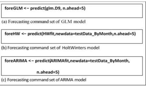
We generate forecasting models by using 3 traditional time series forecasting models, then use all 3 models to forecast power distribution unit in the next 5 intervals from January 2015 to May 2015. After that, we take the predicted values to calculate RMSE and MAPE by comparing with actual values using the R command set in figure 6. The result of experiments is shown in table 1.

Fig. 6. Forecasting command set in R language for traditional time series model

TABLEI

PREDICTED VALUE AND ERROR FOR TRADITIONAL TIME SERIES MODELS

Value Jan Feb Mar Apr May RMSE MAPE

Actual Value 745.82 853.60 1017.89 1100.93 1216.77 - -

GLM 986.13 988.18 990.24 992.3 994.36 166.07 15.78

HoltWinters 841.78 928.33 1000.99 1066.63 1086.62 81.48 7.42

ARIMA 799.24 859.33 969.4 1065.12 1117.63 57.18 4.80

(b) InputTraining

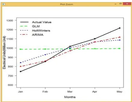
Fig. 7. Comparison graph between 5 intervals of actual value and predicted value

Fig. 8. Function auto.arima() for defining format of ARIMA model

From table 1, the lowest RMSE and MAPE are obtained from ARIMA model. RMSE is 57.18 and MAPE is 4.80. Figure 7 presents a linear plot of actual against predicted values that are obtained from all 3 models. A graph of ARIMA shows the smallest difference between the actual and predicted values. This result is obtained from using auto.arima() for defining ARIMA model as shown in figure 8.

The forecasting ARIMA model consists of autoregressive(AR) in which p = 1 and seasonal autoregressive(SAR) with P = 1. When estimating the coefficientof AR1( )and SAR1( ), we get the values of 0.7301 and 0.6403, respectively, and the parameters d = D = 0 and q = Q = 0. The forecasting equations are presented as follows:

, while is constant

From existing observed values of time series, = 92.42 and the forecasting equation of ARIMA can be present as equation 12.

(12) B. Results of Artificial Neural Networks Model

We define 4 different ANN models: 3L-4N (one neuron in hidden layer), 3L-5N (two neurons in hidden layer), 3L-6N (three neurons in hidden layer), and 3L-7N (four neurons in hidden layer).

From our experiment, we discover that we should not set the goal an error parameter (net.trainParam.goal) too low because it may cause over-fitting. Thus, we set goal error equal to 0.0001. In addition, when we set the initial weight and bias of each

model appropriately, RMSE and MAPE of each model are decreased. As a result, the lowest RMSE and MAPE of each model have been observed after experimentally set the most appropriate parameter values. Theseappropriate initial weights and bias of each model can be summarized in the table 2.

While using initial weight and bias of each model in table 2 to perform model training, then predict next 5 interval of power distribution unit from January 2015 to May 2015. After that, calculate RMSE and MAPE comparing with actual value. We summarize the result in table 3.

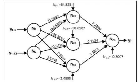
From table 3, we can see that 3L-6N model resulted in the lowest MAPE and table 4 shows that 3L-6N has the highest correlation coefficient. That means the 3L-6N model is highly related to the target. Figure 9 presents a regression graph between the output and the target of a 3L-6N model. When we increase 1 number of neuron, from 6N to 3L-7N, the RMSE and MAPE increase. Therefore, the 3L-6N model is the most appropriate model for predicting this time series. When we use command set in Matlab to show the weight values of each layer, we can define the structure of ANNs as shown in figure 10.

TABLEII

INITIAL WEIGHTS AND BIAS OF EACH MODEL

Model net.iw{1,1} net.lw{2,1} net.b{1} net.b{2} 3L-4N [0.5 0.5] [0.5] [0.5]' [0.5]'

3L-5N [0.5 0.5;0.1 0.1] [0.4 0.4] [0.5 0.5]' [0.5]'

3L-6N [0.5 0.4;0.5 0.5;0.5 0.5] [0.5 0.5 0.5] [0.5 0.5 0.5]' [0.5]'

3L-7N [0.5 0.4;0.5 0.5;0.5 0.5;0.5 0.5] [0.5 0.5 0.5 0.5] [0.5 0.5 0.5 0.5]' [0.5]'

TABLEIII

ACTUAL VERSUS PREDICTED VALUES OF ANNS MODELS Jan Feb Mar Apr May RMSE MAPE Actual Value 745.82 853.60 1017.89 1100.93 1216.77 - -

3L-4N 786.94 789.21 911.85 1096.59 1190.53 59.67 5.21

3L-5N 785.26 809.44 905.99 1123.58 1193.65 58.47 5.08

3L-6N 753.33 816.63 890.15 1148.87 1207.41 63.46 4.58

3L-7N 759.61 760.58 913.55 1089.92 1184.74 64.66 5.33

TABLEIV

CORRELATION COEFFICIENT AND EQUATION OF ANNS

Model Correlation coefficient (R) Relative equation of outputand target

3L-4N 0.84323 Output=0.71*Target+0.16

3L-5N 0.87184 Output=0.76*Target+0.14 3L-6N 0.88868 Output=0.79*Target+0.12 3L-7N 0.84950 Output=0.72*Target+0.16

Fig. 10. Artificial neural networks for 3L-6N model

C. Comparison Between ARIMA and 3L-6N ANN Models

From the literature review [5],[6], the authors suggest that ARIMA is the accurate model to forecast data with moving by trend and season. We thus compare ARIMA with tripple exponential smoothing technique using HoltWinters model and simple linear regression using GLM model. From our experiment, we discover that the ARIMA model gives the lowest error (RMSE = 57.18 and MAPE = 4.80).

To perform time series analysis with ANNs technique, we have found that the 3L-6N model gives the lowest MAPE (=4.58) and also the highest correlation coefficient. That means the output of a 3L-6N model relates the most to the target.

When plot 5 intervals from January 2015 to May 2015 of actual observation values compared to data predicted by ARIMA and 3L-6N models (table 5 and figure 11), it can be concluded that ARIMA’s graph is more similar to the actual observed values than 3L-6N’s graph but a 3L-6N model can adjust irregular error in March to normal error rapidly. As a result, MAPE of 3L-6N is lower than ARIMA but RMSE is higher than ARIMA.

TABLEV

ACTUAL VSPREDICTED VALUES OF ARIMA AND 3L-6NANNMODELS

Value Jan Feb Mar Apr May RMSE MAPE

Actual Value 745.82 853.60 1017.89 1100.93 1216.77 - -

ARIMA 799.24 859.33 969.4 1065.12 1117.63 57.18 4.80

3L-6N 753.33 816.63 890.15 1148.87 1207.41 63.46 4.58

Fig. 11. Comparison graph between ARIMA and ANNs 3L-6N

V. CONCLUSIONS

We study time series analysis for forecasting power distribution unit using monthly data reported by the Metropolitan Electricity Authority from January 2010 to May 2015. We use data from January 2010 to December 2014 as a training set and data form January 2015 to May 2015 as the test set. In our experiment for model comparison, we select 3 traditional time series models (GLM, HoltWinters, ARIMA) and 4 ANNs models (3L-4N, 3L-5N, 3L-6N, 3L-7N).

In traditional time series analysis, ARIMA model is the most accurate model (RMSE = 57.18 and MAPE = 4.80). In ANNs technique, we discover that 3L-6N model (three-layer feed-forward back propagation neural network) is the most appropriate model (MAPE = 4.58, correlation coefficient = 0.88868). When compare ARIMA against the 3L-6N model, it turns out that ARIMA’s graph is more similar to the actual observed values than the 3L-6N’s graph, but MAPE of 3L-6N is lower than ARIMA’s MAPE. As a result, predicted values from 3L-6N model are more accurate than the ARIMA model.

In conclusion, the ANNs model of the 3L-6N structure can be applied to time series forecasting at high precision. The caution is that the high number of hidden layer’s neurons may cause over-fitting.

REFERENCES

[1] Metropolitan Electricity Authority. (2015). Report of electrical distribution [Online]. Available : http://www.mea.or.th/download/index.php# [2] D.W. Bunn and E.D. Farmer, Comparative Models for Electrical

Load Forecasting. New York: John Wiley and Sons, 1985.

[3] P. M. Maçaira, R. C. Souza and F. L. C. Oliveira, “Modelling and Forecasting the Residential Electricity Consumption in Brazil with Pegels Exponential Smoothing Techniques”, Procedia Computer

Science, vol.55, pp. 328-335, 2015.

[4] I. Keka and M. Hamiti, “Load profile analyses using R language” in Proceedings of the ITI 2013 35th Int. Conf. on International

Technology Interfaces, Cavtat, Croatia, 2013, pp. 245-250.

[5] P. Chujai, N. Kerdprasop and K. Kerdprasop, “Time series analysis of household electric consumption with ARIMA and ARMA models” in Proceedings of the International MultiConference of Engineers and

Computer Scientists, Hong Kong, China, 2013, pp. 295-300.

[6] X. Wang and M. Meng, “A Hybrid Neural Network and ARIMA Model for Energy Consumption Forecasting” JOURNAL OF

COMPUTERS, vol.7, No.5, pp. 1184-1190, 2012.

[7] M. Firata, M.E. Turanb and M.A. Yurdusev, “Comparative analysis of neural network techniques for predicting water consumption time series” Journal of Hydrology, vol.384, pp. 46-51, 2010.

[8] I. Boldina and P.G. Beninger, “Strengthening statistical usage in marine ecology: Linear regression” Journal of Experimental Marine

Biology and Ecology, vol. 474, pp. 81-91, 2016.

[9] V. Prema, and K.U. Rao, “Development of statistical time series models for solar power prediction” Renewable Energy, vol. 83, pp. 100-109, 2015.

[10] Y. Wang, J. Wang, G. Zhao and Y. Dong, “Application of residual modification approach in seasonal ARIMA for electricity demand forecasting: A case study of China” Energy Policy, vol.48,

pp. 284-294, 2012.