Abstract—This paper studies the optimal plan for inspection and maintenance of steel structural components in tension by uniform corrosion, considering the following: A deteriorating model uncertain in time is considered, the probability to detect damage during the inspections is modeled, if damage is detected, the structural component is repaired, the failure probability of the component over time is considered supposing that the demands and capacities are random in time, the optimal plan will be the one in which the expected costs (costs of inspection, repair and failure) are minimum in the life cycle of the component, allowing to detect the number of inspections that minimize the expected costs; to determine the optimal plan, all the possibilities that are given of the tree diagram are studied, where each inspection has two existent possibilities: repair or not to repair, the occurrence possibility of each branch in the resulting tree diagram is calculated. In addition, the influence of the variables and parameters are calculated as: the net discount rate of money (r), uniform corrosion rate (), the mean load (T), failure costs (Cf), repair cost (Crep)
inspection cost (Cins) and quality of a nondestructive inspection
(0.5). The results indicate that the optimal number of
inspections in the life-cycle of the component is very sensible to each of the parameters involved. Every parameter in an optimization study needs to be carefully analyzed in order to proceed.
Index Terms—Optimal Inspection, Risk-Based Maintenance, Corrosion Damage, Parametric Analysis
I. INTRODUCTION
HE integrity of offshore platforms, oil ducts, gas ducts, electric power towers, bridges, etc., of steel when confronting corrosion depends strongly on the integrity of the components that form the structural systems [1], [2]. Therefore, it is of high relevance to study the deterioration in time and the means to reduce risks in these structural systems; there are very important contributions of optimal inspection and maintenance [3] – [6]. An optimal inspection plan involves several aspects such as: cost and quality of inspection, cost and quality of repair, failure costs, capacity and demand of the system, net discount rate, uniform
Manuscript received March 11, 2013; revised and accepted April 02, 2013. The authors would like thank to Polytechnic University of Durango, Mexico (www.unipolidgo.edu.mx) for the financial support to present this article.
Cesar Ortega-Estrada is with the Polytechnic University of Durango, Durango, 34300 Mexico (phone: 618-150-1300; e-mail: [email protected]).
Roobed Trejo is with the Polytechnic University of Durango, Durango, 34300 Mexico (e-mail:[email protected]).
David De Leon is with the Autonomous University of Mexico State, Toluca, Mexico, Mexico (e-mail: [email protected]).
Dante Campos is with Mexican Institute of Petroleum, Mexico, D.F., Mexico (e-mail: [email protected]).
corrosion rate, time for corrosion initiation, etc. The fundamental problem is to determine the optimal number of inspections in the lifetime of the component considering the indicated aspects, but also maintaining a certain level of reliability, which has been previously specified.
In previous papers, repair has been considered flawless; this means that after the repair, the same initial properties are obtained, for example in [7], repair is considered to be perfect when accumulated damage by earthquakes in buildings is intervened. In other papers like [4], inspection and maintenance are considered imperfect, and for the specific case of damage by corrosion in steel rebars embedded in reinforced concrete elements, it is considered that after repair, the reliability of structural component increases, but the original conditions are not regained.
In the specific case of damage by uniform corrosion, the material is lost overtime, what produces a reduction in the transversal section of steel structural member. This paper considers the effect of uniform corrosion on a steel component, considering that the only option of repair is cleaning and applying an anticorrosive paint as indicated in the standards. Therefore, after repair, there is not a greater reliability of the component because the repair does not restore the material lost by corrosion.
II. LIFECYCLECOST
In the last two decades, mathematical models that calculate the life cycle of members and structural systems have been proposed, for example, [4], [7] - [9]. This article follows the methodology proposed in [4] with two main differences: (1) Repair consists in cleaning the component and applying anticorrosive paint, therefore, after repair, the probability of failure does not decrease, This helps to model the real effect of repair. And (2) all the repair possibilities are evaluated in a tree diagram (based on a computer software), where the following aspects are considered explicitly: quality of inspection costs of inspection, repair and failure, the growing effect of uniform corrosion. It is considered in a realistic way the repair effect on the reliability of the component damaged by corrosion; and the effect of the value of money over time.
This paper assumes a circular cross-sectional tubular steel element with tension load under the following parameters:
1. Life-cycle Time (L) = 20 years 2. Exterior Diameter (D0) = 102 mm
3. Interior Diameter (d0) = 90.52 mm
Optimal Plan for Inspection and Maintenance of
Structural Components by Corrosion
Cesar Ortega-Estrada, Roobed Trejo, David De Leon and Dante Campos
4. Mean Tension Load (T) = 43.74 t
5. Coefficient of Variation for Load (CVT) = 0.25 6. Mean Yield Stress (fy) = 4620 kg/cm2 7. Coefficient of Variation for fy (CVfy) = 0.1 8. Annual Increment for CVfy = 0.02
9. Corrosion Initiation after applying the anticorrosive paint. (Tic) = 3 years
10. Corrosion Rate () =0.0089 cm/year
11. Damage intensity at which the method of inspection has a 50% of detection probability (0.5) = 0.1
12. Coefficient of Variation for Inspection (CV0.5) = 0.333
13. Annual discount rate (r) = 0.05 14. Inspection Cost (Cins) = 500 ($USD) 15. Repair Cost (Crep) = 3,000 ($USD) 16. Failure Cost (Cf) = 100,000 ($USD)
17. Number of inspections in the Life-cycle (m) = 2
The intensity of damage is evaluated as it is indicated as in (1), where D(t) is the exterior diameter of the member over time t; before of the first repair, the exterior diameter is estimated as shown in (2a) and (2b), after the first repair occurs, it is calculated as shown in (3a) and (3b), where DR is the exterior diameter of the member when repairing overtime tR.
(1)
for (2a)
for (2b)
for (3a)
for (3b) In [4] the probability to detect damage d() is calculated as in (4), where min is the minimum detectable intensity damage and max is the intensity of damage when the probability of detection is 1. Notice that the probability to detect damage depends on the mean and the standard deviation of the intensity of damage that a certain inspection method detects.
for (4a)
for (4b)
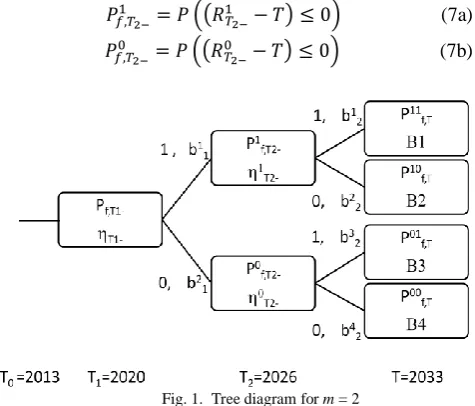
for (4c) To represent all the possible events associated with repair and non-repair actions, a tree event analysis is performed. From this moment on, Fig. 1 is considered to be the tree diagram for two uniformly distributed inspections in the life cycle of the component (m = 2), where 0 and 1 represent actions on repair and non-repair, respectively. Ti is the time of inspection; bji represents the corresponding event of occurrence of the branch j overtime Ti; the probability of failure of the component before the first inspection is estimated with (5), where T represents the random variable of the tension load and RT1- is the resistance of the
component before the first inspection.
(5) According with [4], the probability of the event b11 is calculated with (6) where T1- is calculated with (1).
(6)
The probability of failure of the component before the second inspection, given the branch b11, is calculated with (7a); and for the branch b21, with (7b).
[image:2.595.312.550.224.427.2](7a) (7b)
Fig. 1. Tree diagram for m = 2
After the second inspection, given the occurrence of the event b11, there are two possibilities, b12 and b22, that indicate the action to repair or not to repair. In the same way, given the occurrence of the event b21, there are two possibilities b32 and b42, which also indicate the action to repair or not to repair [4].
(8a)
(8b)
Each branch in the tree represents a sequence of events
bji. If all the events bji are independent, see [4], the probability of occurrence of the trajectories B1, B2, B3 and B4 can be calculated with (9a), (9b), (9c) and (9d) respectively.
(9a)
(9b)
(9c)
(10a) (10b) (10c) (10d) Each branch has tree probabilities of failure (before the first inspection, before the second inspection, and at the end of its life time cycle); the probability of failure for each branch is calculated with (11a), (11b), (11c) and (11d).
Fig. 2. Evolution of the probability of failure for all the possibilities of repair if m = 2
(11a) (11b) (11c) (11d) The probability of failure in the life on the component is:
(12) The optimal maintenance plan is that in, which the costs of inspection, repair, and failure are minimum. The costs of inspection are calculated with (13), where Cins is the cost of inspection based on the employed technique. The costs of repair are calculated with (14a), where Crep is the cost of repair based on the method used. The costs of failure are estimated with (15), where Cf are the consequences of failure. The total cost is calculated with (16).
(13)
(14a) (14b)
(15)
(16)
III. OPTIMAL INSPECTION PROGRAM
To calculate the life cycle costs, great effort is required; therefore, a computer software was developed OIMS v01 [10] and [11]. The method was followed for the data presented considering a variation in the number of inspections (m = 0, 1, 2, 3, 4, 5, 6, 7, 8, 9 and 10), the results
[image:3.595.59.297.193.443.2]are presented in Fig. 3. The optimal number of inspections resulted to be m = 5, and the branch with the greatest probability of occurrence is 00011; Fig. 4 shows the evolution of the probability of failure of that branch.
[image:3.595.318.541.292.437.2]Fig. 3. Optimization Costs in function of the number of inspections with uniform intervals in the life time cycle.
Fig. 4. Evolution of the probability of failure for the trajectory 00011 if m = 5
IV. PARAMETRIC ANALYSIS
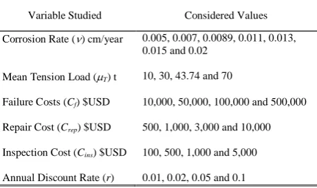
It is of major interest, to evaluate the importance that each variable has in the determination of the optimal number of inspections in the life time cycle of the component at issue. The variables analyzed are presented in Table 1.
TABLEI
VARIABLES CONSIDERED IN THE PARAMETRIC STUDY
Variable Studied Considered Values
Corrosion Rate () cm/year 0.005, 0.007, 0.0089, 0.011, 0.013, 0.015 and 0.02
Mean Tension Load (T) t 10, 30, 43.74 and 70
Failure Costs (Cf) $USD 10,000, 50,000, 100,000 and 500,000
Repair Cost (Crep) $USD 500, 1,000, 3,000 and 10,000
Inspection Cost (Cins) $USD 100, 500, 1,000 and 5,000
Annual Discount Rate (r) 0.01, 0.02, 0.05 and 0.1
The effect of the Corrosion Rate () is shown in Fig. 5; if increases, the optimal number of inspections in the life-cycle of the component increases too. Notice that the optimal number of inspections is very sensible between = 0.005 and 0.0089 cm/year. In real cases, corrosion rates between these intervals have been found [12]. The tags shown in Fig. 5 represent , calculated for each case.
0 0.02 0.04 0.06 0.08 0.1 0.12 0.14 0.16
2013 2014 2015 2016 2017 2018 2019 2020 2021 2022 2023 2024 2025 2026 2027 2028 2029 2030 2031 2032 2033
P
ro
b
ab
ili
ty
o
f f
ai
lu
re
Year
00
01
10
11
0 2,000 4,000 6,000 8,000 10,000 12,000 14,000 16,000
0 1 2 3 4 5 6 7 8 9 10
C
o
st
s
($
U
S
D)
Number of inspections (m)
Inspection Cost Repair Cost Failure Cost Total Cost m = 5
0 0.01 0.02 0.03 0.04 0.05 0.06 0.07
2013 2014 2015 2016 2017 2018 2019 2020 2021 2022 2023 2024 2025 2026 2027 2028 2029 2030 2031 2032 2033
P
ro
b
a
b
il
it
y
o
f
fa
il
u
re
[image:3.595.313.544.555.692.2]Fig. 5. Optimal number of inspections in function of the corrosion rate (cm/year).
The Mean Tension Load (T), in the optimal number of inspections is shown in Fig. 6. The allowed tension for the studied member is 43.74 t and the optimal number of inspections is 5. If the mean tension load is reduced to 30 t (an approximate reduction of 31%), the optimal number of inspections is 0; therefore, the optimal number of inspections is very sensible to the load level in the system.
Fig. 6. Optimal number of inspections in function of the mean load (t).
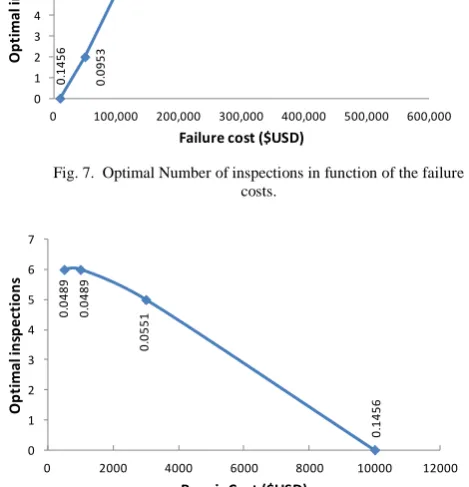
The consequences of failure also have great influence in the determination of the optimal number of inspections in the life time cycle, Fig. 7 presents the results of the parametric analysis, where it can be observed that it is very important to determine in detail the consequences of failure, where direct loss must be considered (production loss, installation damage, environment damage, injury or loss of human life) and also indirect loss (other industrial sectors will have lost because the sector that provides the goods or services are out of service); in this topic, very few studies have been done so it is justifiable to deepen into the determination of the failure consequences.
[image:4.595.52.287.63.196.2]The costs of repair also have a great influence in the determination of the optimal number of inspections. Fig. 8 shows that if the cost of repair reduces, then the optimal number of inspections increases, in other way, if the cost of repair increases, then the number of inspections reduces.
[image:4.595.313.548.113.357.2]Fig. 7. Optimal Number of inspections in function of the failure costs.
Fig. 8. Optimal Number of inspections in function of the repair costs.
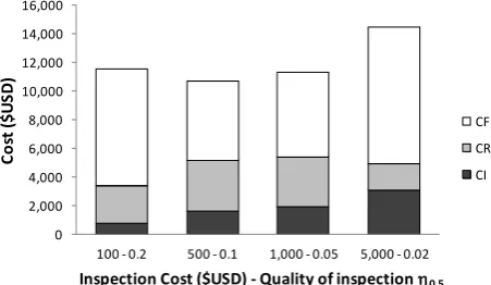
Figure 9 shows the influence of the inspection costs with the optimal number of inspections. In this case, there is a direct relation between the costs of inspection and the quality of inspection. This work supposes that when the cost of inspection increases, the detectable intensity of damage decreases (represented by a 50% probability of detection 0.5).
Figure 10 presents the costs associated to different alternatives of cost and quality of inspection, so the alternative with the minimal cost can be visualized. This type of analysis helps to determine when to inspection and with what inspection technique, minimizing the costs.
Fig. 9. Optimal Number of inspections in function of the costs and quality of inspection.
0 .0 4 8 8 0 .0 6 7 1 0 .0 5 5 1 0 .0 6 2
3 0.0
5 7 9 0 .0 6 1 0 0 .0 7 7 5 0 1 2 3 4 5 6 7
0 0.005 0.01 0.015 0.02 0.025
O p ti ma l I n sp ec ti o n s
Corrosion rate (cm/year)
0 .0 0 0 0 0 .0 0 5 5 0 .0 5 5
1 0.5
4 1 8 0 1 2 3 4 5 6 7
0 10 20 30 40 50 60 70 80
O p ti ma l i n sp ec ti o n s
Mean Load (t)
0 .1 4 5 6 0 .0 9 5 3 0 .0 5 5 1 0 .0 4 3 4 0 1 2 3 4 5 6 7 8 9 10
0 100,000 200,000 300,000 400,000 500,000 600,000
O p ti ma l i n sp ec ti o n s
Failure cost ($USD)
0 .0 4 8 9 0 .0 4 8 9 0 .0 5 5 1 0 .1 4 5 6 0 1 2 3 4 5 6 7
0 2000 4000 6000 8000 10000 12000
O p ti ma l i n sp ec ti o n s
Repair Cost ($USD)
0 .0 8 2 1 0 .0 5 5 1 0 .0 5 8 9 0 .0 9 5 8 0 2 4 6 8 10 12 14
100 - 0.2 500 - 0.1 1,000 - 0.05 5,000 - 0.02
O p ti ma l i n sp ec ti o n s
[image:4.595.315.548.229.365.2] [image:4.595.58.287.340.473.2] [image:4.595.319.545.564.695.2]Fig. 10. Associated costs to the Optimal Number of Inspections in function of the costs and quality of inspection.
[image:5.595.59.284.313.449.2]Fig. 11 presents the optimal number of inspections in function of the annual discount rate (r). The obtained results agree with [8]. The annual discount rate must be a realistic factor in an optimization study, because it also influences in the determination of the optimal number of inspections in the life cycle of the component.
Fig. 11. Optimal number of inspections in function of the annual net discount rate.
V. CONCLUSIONS
This article presents the methodology to calculate the optimal number of inspections in a steel member with cross-sectional tubular circular subject to tension load, under the effect of uniform corrosion. When calculating the optimal number of inspections, all the possible events associated with actions of repair and non-repair are considered; the following aspects are explicitly considered: cost and quality of inspection, failure consequences, demand and capacity of the system, net discount rate, deterioration rate and initiation of damage overtime. The type of repair-maintenance considered is only the replacement of the anticorrosive paint, so after repair, there is no decrease in the probability of failure.
Also, a parametric study on the following variables was preformed: Corrosion Rate (Mean Tension Load (T), Failure Cost (Cf), Repair Cost (Crep), Inspection Cost (Cins) and Annual Discount Rate (r). Important results were obtained, because the optimal number of inspections in fact is sensible to the values adopted by each one of the variables, therefore, the optimization studies must justify in a realistic way each one of the adopted values.
The methodology presented helps to determine when to inspection and with what inspection technique, minimizing the costs on the life-cycle.
ACKNOWLEDGMENT
The results presents in this paper are part of the doctoral thesis of the first author for the Faculty of Engineering of the Autonomous University of Mexico State, Mexico (www.uaemex.mx).
REFERENCES
[1] Alamilla, J.L., De Leon, D., and Flores, O., “Reliability based integrity assessment of steel pipelines under corrosion”. Corrosion Engineering, Science and Technology, Maney Publishing, Vol. 40, No. 1, 2005, 69-74.
[2] Biezma, M.V., and Schanack, F., “Collapse of Steel Bridges.” Journal of Performance of Constructed Facilities, ASCE, Vol. 21, No. 5, 2007, 398-405.
[3] Mori, Y., and Ellingwood, B.R., “Maintaining reliability of concrete structures. II: Optimum inspection/repair.” Journal of Structural Engineering, ASCE, 120(3), 1994, 846-862.
[4] Frangopol, D.M., Lin, K.Y., and Estes, A.C., “Life-cycle cost design of deteriorating structures.” Journal of Structural Engineering, ASCE, 123(10), 1997, 1390-1401.
[5] Nielsen, J.J., and Sorensen, J.D., “On risk-based operation and maintenance of offshore wind turbine components.” Reliability Engineering and System Safety, ELSEVIER, Vol. 96, 2011, 218-229. [6] Straub, D., and Faber, M.H.,. “Computational Aspects of Risk-Based
Inspection Planning”. Computer-Aided Civil and Infrastructure Engineering. Blackwell Publishing, Vol. 21, 2006, 179-192. [7] Esteva, L., Campos, D., and Diaz-Lopez, O., “Life-cycle optimization
in earthquake engineering.” Structure and Infrastructure Engineering, Taylor and Francis, Vol. 7, No. 1-2, 2011, 33-49.
[8] Thoft-Christensen, P., “Life-cycle cost-benefit (LCCB) analysis of bridges from a user and social point of view.” Structure and Infrastructure Engineering, Taylor and Francis, Vol. 5, No. 1, 2009, 49-57.
[9] Ang, A. H.-S., and De Leon, D., “Modeling and analysis of uncertainties for risk-informed decisions in infrastructures engineering.” Structure and Infrastructure Engineering, Taylor and Francis, Vol. 1, No. 1, 2005, 19-31.
[10] Ortega-Estrada, C., and Trejo, R., “Optimal Inspection and Maintenance of Structures.” Theory Manual OIMS v01. 2013 [11] Trejo, R., and Ortega-Estrada, C., “Optimal Inspection and
Maintenance of Structures.” User Manual OIMS v01. 2013
[12] Melchers, R.E., “Examples of mathematical modeling of long term general corrosion of structural steels in sea water” Corrosion Engineering, Science and Technology, Maney Publishing, Vol. 41, No. 1, 2006, 38-44
0 2,000 4,000 6,000 8,000 10,000 12,000 14,000 16,000
100 - 0.2 500 - 0.1 1,000 - 0.05 5,000 - 0.02
C
o
st
($
U
S
D
)
Inspection Cost ($USD) - Quality of inspection 0.5 CF
CR
CI
0
.0
7
7
2 0.0
6
4
1 0.0
5
5
1 0.0
4
8
9
0 1 2 3 4 5 6 7
0 0.02 0.04 0.06 0.08 0.1 0.12
O
p
ti
ma
l i
n
sp
ec
ti
o
n
s