Performance Characteristics Comparison of ANN & ANFIS controller
for PMSG Variable Speed WECS
V.LAKSHMA NAIK1, Dr.R.KIRANMAYI2
1
Research Scholar, Dept of EEE, JNTUCEA, Ananthapuramu, Anantapur (Dt), AP, India, 2
Professor & HOD, Dept of EEE, JNTUCEA, Ananthapuramu, Anantapur (Dt), AP, India,
Abstract--This paper mainly deals with the WECS, using PMSG. To overcome the demerits and the draw backs occurred in these systems. a new DC Optimal level Reference standard, however maximum power point tracking algorithm also used to obtain the new optimal operating point for the power curve. This optimal operating point is depends upon DC INTERLINK VOLTAGE and currents. The proposed ANN and ANFIS technique is simulated in mat lab/ Simulink software. Here the WECS is evaluated and compared with conventional ANN and ANFIS network methods. The problems related with the Power Co-Efficient , the TIP SPEED RATIO and DC inter link voltage and average power is evaluated over the total power extraction of WECS has provided with the modern advantages with all these errors consideration and improvement. As extension of this system we used the ANIFS system to grid side connection for the control purpose. This control signal also derived in order to achieve MPPT along with this the Total Harmonic distortion is also calculated for all mentioned systems.
Key words: WECS, PMSG, ANN, ANFIS, MPPT, TSR, PSF, HCL, THD.
I.INTRODUCTION
The wind energy Generation system (WGS) can broadly classified into two types i).A constant-speed wind turbine(CSWT) which is based on fine tuning of the pitch angle of wind turbine blades. It is such that the output power extraction from the wind is controlled. ii).A Variable- speed wind turbine (VSWT) with optimum tip speed ratio (TSR). Compare to constant speed wind turbine the variable speed wind turbine are more striking. As they can extract maximum power at various wind velocities and they also decreases the Mechanical stress on the Wind Energy Conversion System (WECS). The pitch control technique which is used in the constant–speed wind turbine generator developed with a non- linear model of Permanent Magnet Synchronous Generator (PMSG). Alternatively we can use inverse system method which can control the output power over a wide range, but the non parametric uncertainties will cause the problems. In the proposed papers the torque ripples of PMSG are also reduced using electro-mechanical analyses. This will increase the machine efficiency, but the analysis doesn’t revel about optimum power extraction in PMSG.
The conventional constant-speed WECS using squirrel cage Induction Generator (SCIG) or Double Fed Induction Generator (DFIG), but the energy supplied to the load is does not track the Maximum
power point (MPPT). The MPPT control technique is commonly implemented in order to change the wind energy into electrical energy at higher efficient levels, in the wind power generation system (WPGS). In this paper we are studying about the variable speedWECS. For MPPT in WECS having three main algorithms are i).TSR ii).Power signal feedback (PSF) iii).Hill Climbing Search method. But these traditional technique used in WESC is having there own problems such as i).High Frequency Jitter ii).Low Precision and iii).Estimation levels of faults also falls down. There are many more active techniques are desperately trying to get MPPT point for WECS at higher standard levels. At present three main technique which are mainly used for MPPT in WECS i).Hill climbing technique ii).Wind speed measurement (WSM) iii).PSF.
In proposed paper the computer intelligence (CI) method used along with the Adaptive Neuro Fuzzy Inference System (ANFIS). In this paper the optimistic challenging issues such as Transient, Sub-Transient and Steady state conditions are also considered.
II. METHODOLOGY A. Modeling of PMSG with Wind Turbine.
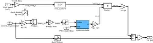
The below simulation shows how the PMSG is modeled with the wind turbine. Generalized model has been derived. Now a day’s wind system operation is widely being worked out so as to extract maximum active power at all possible wind speeds with least detrimental effects on overall performance. In a fixed speed wind turbine system (FSWTS), the generator rotates at an almost constant speed for which it is designed regardless of variation in wind speed.
As a result, the turbine will be the most efficient in extracting the maximum power from the wind for
only one particular wind speed and wasted significant amount of energy. Also as turbine is forced to operate at constant speed, it necessary for the turbine to be extremely robust to withstand a significant amount of mechanical stress due to the wind speed fluctuations On the other hand with VSWTS, the rotor of the generator is allowed to rotate freely. Thus, it is possible to control the rotor speed by the means of power electronics to maintain the optimum TSR at all times under varying wind conditions. Several different configurations are researched and developed like fixed speed system with a SCIG, variable speed system with PMSG and DFIG to improve the efficiency While recent research has considered larger scale designs, the economics of large volumes of permanent magnet material has limited their practical application. But now a day’s as cost of magnet has fallen down in global market significantly, PMSG WT has become most preferred system for wind generation. The primary advantage of PMSG is that they do not require any external excitation current. A major cost benefit in using the PMSG is the fact that a thyristor bridge rectifier may be used at the generator terminals since no external excitation current is needed. Further, the elimination of the gear box and brushes can increase the efficiency of wind turbine by 10%.
Hence wind turbines generators based on PMSG without gear box is more useful over electrically excited machines The simulation results show that given PMSG wind turbine design can be extended for grid connection. Output power and voltage of WECS gets effectively smoothed using proposed method PMSG was wound-field synchronous machines require DC current excitation in the rotor winding. This excitation is done through the use of brushes and slip rings on the generator shaft. However, there are several disadvantages such as requiring regular maintenance, cleaning of the
carbon dust, etc. An alternative approach is to use brushless excitation which uses permanent magnets instead of electromagnets.
Fig.1 Wind Schematic Diagram Based On PMSG Power extracted from the wind turbine.
Pm =0.5 π ρCp (λ, β )R2 (vw
The aerodynamic efficiency of a wind turbine is described by the power coefficient function, Cp (β, λ) given by,
Cp=(Pm/Pw)
Wind turbine is applied to convert the wind Energy to mechanical torque. The mechanical torque of turbine can be calculated from mechanical power at the turbine extracted from wind power. This fact of the wind speed after the turbine isn’t zero. Then, the power coefficient of the turbine (Cp) is used. The power coefficient is function of pitch angle (β) and tip speed (λ), pitch angle is angle of turbine blade whereas tip speed is the ratio of rotational speed and wind speed. The power coefficient maximum of (Cp) is known as the limit of Betz. The power coefficient is given by:
= -
The Cp-λ characteristics, for different values of the pitch angle β, and for different values tip speed ratios.
Cp=(Pm/Pw)
The total power extracted from the wind is. Pm =0.5 π ρCp (λ, β )R2 (vw )2 The mechanical torque is given by,
Tm =
Fig. 2 MATLAB/Simulink Model for Wind Turbine
B. Modeling of PMSG.
The voltage equations of PMSG are given by: id = Vd - id - P ωr iq
iq = Vq - iq - P ωrid - The electromagnetic torque is given by:
Te = 0 .75ρ[ λiq - ) id iq] The dynamic equations are given by,
= (Te -F ωr - Tm) ωr
Fig. 3 Modeling Of PMSG Using Mathematic Equations for Electromagnetic Torque.
Fig. 4 Modeling of PMSG Using Mathematic Equations for Rotor Speed and Rotor Angle.
C. Mathematical Inverse Park and Clark Transform
A practical generator produces 3 phase AC power. For this reason, the inverse Park and Clarke transforms are introduced to implement the 3 phase AC output from the generator model. As Fig 2.5 shows, the transform from the stator axis reference frame (α, β) to the rotating reference frame (d-q) is called the Park transform (Texas Instruments 1997). The Clarke transform is the transformation of the 3- phase reference frame to the 2- phase orthogonal stator axis (αβ).
Fig. 5 Inverse Park Transformation.
As of Fig.3 illustration, assumes the αβ frame has an angle θ Field with the dq frame, the inverse Park transform (dq - αβ) which can be expressed as follows:
D. WECS Using Artificial neural network Controller
For this technique we study all the factors
i).Power Coefficient, ii).TSR, iii).Torque, iv).Speed, v).DC Link Voltage, vi).Active Power Comparison.
ANN Controller:
In this section we are going to study about Artificial Neural Network (ANN) based controller. Here we study all the factors related to the ANN. The training methods used for the neural network. The ANN network is simulated for WECS using Artificial Neural intelligence. Fig.6 shows how exactly the ANN will control the WECS. The fig.6 show only for the model for TSR. Similarly models have been developed for the different control technique.
However the model based on the ANN will give relation:
Pm= (J )+Pe
Information flows through a neural network in two ways. When it's learning (being trained) or operating normally (after being trained), patterns of information are fed into the network via the input units, which trigger the layers of hidden units, and these in turn arrive at the output units. This common design is called a feed forward network. Not all units "fire" all the time.
Each unit receives inputs from the units to its left, and the inputs are multiplied by the weights of the connections they travel along. Every unit adds up all the inputs it receives in this way and (in the simplest type of network) if the sum is more than a certain threshold value, the unit "fires" and triggers the units it's connected to. The different control techniques which are used to train ANN are feed forward network and back propagation network. Let us study each every factor in detail
Fig.6 ANN based Controller for MPPT
Block Diagram:
This ANN code is used for the setting up of reference voltage in dc link. On basis of this we are getting control signal for converter models. Further they are fed to the signals which are used for control signals. The block diagram of the proposed model is as shown below.
Fig.7 Block Diagram of the Proposed Paper. As above diagram shown the basic objective of the project is to achieve complete control over the WECS. To achieve this object we used completely modeled PMSG with variable speed turbine. Using actual wind speed and reference wind speed we develop the converter controller model. However we are developing the controlling technique on both sides. But the main concentration is at inverter section or grid side. The variable speed turbine generator produce more efficiency when compare to the constant speed turbine generator.
The ANN code uses DC current and DC voltage as input signal and get best possible signal as output
signal. Here each the position and velocity vectors of the input vectors initialized randomly. Here each parameters are considered as the different particle, which is allowed reach its best value that is pbest. Then it will compare with the global best and den start converges at gbest value. Along with this we also utilized some of the constrain function. Each parameter is allowed to achieve the fitness function then they are compared.
Fitness function = max(Pd) Dc power is achieved by:
Pd = ( Vdc*Idc) Therefore optimal output is achieved by comparing the above formula. This is the first step to achieve maximum efficiency. The actual working ANN code is given below. Which is used for the achieving the required reference level.
irk+1 = w * + 1 *rand1 *( - ) *
+ 2 * rand2 ( - )
= + The 𝑉𝑖𝑘 must be specified in the maximum and
minimum range of [vmax, vmin]
III.EXTENSION SYSTEM A.ANFIS Controller.
In this section we are studying about another hybrid technique ANFIS controller. Till to the day it is only applied to rotor section, we will apply this ANN and fuzzy control system to grid section. Here comparison is done along with all remained control technique. The standard ANN is modeled along with the fuzzy rules to achieve the better outputs.
B.Adaptive Neuro Fuzzy Inference System (ANFIS)
Fuzzy Logic Controllers (FLC) has played an important role in the design and enhancement of a vast number of applications. The proper selection of the number, the type and the parameter of the fuzzy membership functions and rules are crucial for
achieving the desired. ANFIS are fuzzy Sugeno models put in the framework of adaptive systems to facilitate learning and adaptation. Such framework makes FLC more systematic and less relying on expert knowledge. To present the ANFIS architecture, let us consider two-fuzzy rules based on a first order Sugeno model.
Rule 1: if (x is A1) and (y is B1), then (f1 = p1x +
q1y + r1)
Rule 2: if (x is A2) and (y is B2), then (f2 = p2x +
q2y + r2)
One possible ANFIS architecture to implement these two rules is shown in Figure. Note that a circle indicates a fixed node whereas a square indicates an adaptive node (the parameters are changed during training).
Layer 1: All the nodes in this layer are adaptive
nodes
Layer 2: The nodes in this layer are fixed (not
adaptive). These are labeled M to indicate that they play the role of a simple multiplier. The output of each node is this layer represents the firing strength of the rule.
Layer 3: Nodes in this layer are also fixed nodes.
These are labeled N to indicate that these perform a normalization of the firing strength from previous layer.
Layer 4: All the nodes in this layer are adaptive
nodes. The output of each node is simply the product of the normalized firing strength.
Layer 5: This layer has only one node labeled S to
indicate that is performs the function of a simple summer.
C. Rules for Expert ANFIS
i.If (mper is Low) and (Lifecycle is Low) then
(Quality_Class is Poor1)
ii.If (mper is Low) and (LifeCycle is High) then (Quality_Class is Good1)
iii.If (ctran3 is High) and (LifeCycle is High) then (Quality_Class is Poor2)
iv.If (ctran3 is Low) and (LifeCycle is High) then (Quality_Class is Good2)
v.If (mtran is High) and (aper is High) and (LifeCycle is High) then (Quality_Class is Poor3) vi.If (aper is Low) and (atran is Low) and (LifeCycle is High) then (Quality_Class is Good3)
D.Membership Function Description
The type of membership functions used in this research work in Gauss2mf. Although some other types of membership functions like gaussmf and trimf were also experimented but gauss2mf function provides better performance. The membership functions in the ANFIS system have 2 stages. In the start the membership functions are at their default shapes .This default shape changes when the ranges are assigned to them. After performing the training the membership functions have a changed shape. The reason for this change is that when an ANFIS undergoes from training process it tunes the membership functions according to the corresponding training data and rules. So membership functions of a trained ANFIS have a different shape as compared to an untrained ANFIS. Another important thing to remember is that the shapes of only those membership functions are changed which are included in any rules.
Fig.9 ANFIS
The fuzzy inference system that we have considered is a model that maps: Input characteristics to input membership functions, input membership function to rules, rules to a set of output characteristics,
output characteristics to output membership functions, and the output membership function to a single-valued output, or a decision associated with the output. We have only considered membership functions that have been fixed, and somewhat arbitrarily chosen. Also, we have only applied fuzzy inference to modeling systems whose rule structure is essentially predetermined by the user’s interpretation of the characteristics of the variables in the model. In general the shape of the membership functions depends on parameters that can be adjusted to change the shape of the membership function. The parameters can be automatically adjusted depending on the data that we try to model but the modeling have certain limitations.
IV.SIMULATION RESULTS
The proposed system is ANFIS controller technique. Here the proposed system is compared the ANN Controller. The no of output factors are also calculated and they are compared. Let start our discussion with PI controller.
A. Simulated Model for ANN Controller
Fig.9 shows the simulated model for wind energy conversion system using Artificial Neural Network controller. Fig.10 shows how exactly the ANN will controltheWECS. The fig.10 show only for the model for TSR. Similarly models have been developed for the different control technique.
Fig.10 Simulated Model of ANN Controller Torque:
Fig.10 shows the simulated torque output of the ANN controller model. In this graph we will observe the Transient period and steady state values of the ANN controller. In fig.11 the graph is plotted between the Electromagnetic Torque and the time. The graph shows that the transient state will be continuing up to 3 sec. until the time space reaches to 3 sec , the torque will be fluctuating . After it reaches to 3 sec the torque become constant. After 8 sec the torque starts falling. Initially the torque will produce too much variation.
Fig.11 Simulated Output Graph of the Torque for ANN Controller.
Tip Speed Ratio:
The fig.12 shows the simulated model output of the PI controller for TSR. The duration for transient state output of the TSR and the time instant when it reaches to steady state value.
Fig. 12 Simulated Output Graph of the Tip Speed Ratio for ANN Controller.
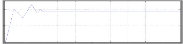
The fig.12 shows the graph plotted between TSR and time. The required tip speed ratio for maximum power point is 12. The graph will start around the 9 and initial sub transient condition may cause the disturbance. After 1 sec the TSR will keep increasing it will reach the study state after 4.5 sec. Rotor Speed:
The fig.13 shows the transient and steady state variation of the rotor speed. The transient state variation the duration which is taken by the controller to reach steady state time period. Initially due to transient condition a certain fluctuation will accrue in rotor speed.
Fig.13 Simulated Output Graph of the Rotor Speed for ANN Controller
It will take 2 sec to transient period to get over. After 2 sec the speed almost remains constant till 9 sec. After that the speed starts falling below nominal value.
DC Interlink Voltage:
Fig.14 shows the simulated waveform of the DC interlink voltage between the converter as well as inverter section. Which is capacitor connected reference voltage, which will set the balance for inverter operation to maintain the reference standards.
Fig.14 Simulated Output Graph of the DC- Interlink Voltage for ANN Controller
The DC Interlink voltage is stared at almost 1600 or 1650 voltage, as the transient valve got over the interlink voltage almost settle down to 1250. The capacitor will get the proper required value of the voltage.
Active Power:
The fig.15 shows the simulated graph of the ANN Controller for active power. From the graph it clears that due to transient condition the power swing will accrue. In this fig only active power is taken into account, because it is the actual amount of the power which is used. By analyzing the graph we observe that the power curve swings between 0.0 to 1.1 during the time period 0 to 1 sec. From t=1 sec the power curve starts to increase slowly. And reaches it .98 MW at t= 4 sec. after the maximum power remains constant at value of 1.75MW. From t=9 sec it start decreasing slowly. These values are
also compared with other ANN and PSO-RNN technique values.
Fig.15 Simulated Output Graph of the Active Power for ANN Controller.
B.Simulation of Extension System
In this section we are studying about another hybrid technique ANFIS controller. Till to the day it is only applied to rotor section, we will apply this ANN and fuzzy control system to grid section. Here comparison is done along with all remained control technique. The standard artificial neural network is modeled along with the fuzzy rules to achieve the better outputs.
Fig.16 Simulated Model of the ANFIS Controller
Torque:
Fig.17 shows the simulated torque output of the ANFIS controller model. In this graph we will observe the Transient period and steady state values of the ANFIS controller
Fig.17 Simulated Output Graph of the Torque for ANFIS Controller
In fig.17 the graph is plotted between the Electromagnetic Torque and the time. The graph shows that the initial transients are high, compare PI
and ANN controlling technique. These transients will be continue up to 3 sec. until the time space reaches to 3 sec , the torque will be fluctuating . After it reaches to 3 sec the torque become constant. Up to 6 sec the torque will holds good. After that it will start falling.
Tip Speed Ratio:
The fig.18 shows the simulated model output of the ANFIZ controller for TSR. The duration for transient state output of the TSR and the time instant when it reaches to steady state value.
Fig.18 Simulated Output Graph of the Tip Speed Ratio for ANFIS Controller
The fig.18 shows the graph plotted between TSR and time. The required tip speed ratio for maximum power point is 12. The graph will start around the 9 Nm, and initial sub transient condition may cause the disturbance. After 1 sec the TSR will keep increasing it will reach the study state after 4.5 sec. This will overlap on the exact value that is used for the maximum operating point.
Rotor Speed:
The fig.19 shows the transient and steady state variation of the rotor speed. The transient state variation are studied and the duration which is taken by the controller to reach steady state time period. According to simulation the speed starts from negative value. During starting few transient will be very high. As time progresses these transients were suppressed. By the end of transient the speed will reach 1 rpm. After 2 sec these transients will vanish out and speed becomes steady as shown in the fig.19
Fig.19 Simulated Output Graph of the Rotor Speed for ANFIS Controller
DC Interlink Voltage:
Fig.20 shows the simulated waveform of the DC interlink voltage between the converter as well as inverter section. Which is capacitor connected reference voltage, which will set the balance for inverter operation to maintain the reference standards.
Fig.20 Simulated Output Graph of the DC interlink voltage for ANFIS Controller
The DC Interlink voltage is stared at almost 1600 or 1650 voltage, as the transient valve got over the interlink voltage almost settle down to 1150. The capacitor will get the proper required value of the voltage. That is constant voltage is maintained as per grid reference value. These reference slandered will done according to the grid section.
Active Power:
The fig.21 shows the simulated graph of the ANFIS Controller for active power. From the graph it clears that due to transient condition the power swing will accrue. In this fig only active power is taken into account, because it is the actual amount of the power which is used.
Fig.21 Simulated Output Graph of the active power for ANFIS Controller.
In the proposed method the real power remains constant over a time period whereas power fluctuations occur in the ANN and PI controller techniques as it is evident from Fig. The superiority of the proposed method over the existing methods in terms of real power is clearly identified. The power
starts to increase gradually from t = 0 sec and reaches its maximum power value of 1MW at t=3sec. After reaching the maximum power, the curve remains steady after t=3 sec. As compared to the power obtained using the other techniques, the proposed method only attained the rated power of 1MW.
C.Total Harmonic Distortion (THD) calculation
The THD of a signal is a measurement of the harmonic distortion present and is defined as the ratio of the sum of the powers of all harmonic components to the power of the fundamental frequency. THD is used to characterize the linearity of audio systems and the power quality of electric power systems. Distortion factor is a closely related term, sometimes used as a synonym.
In audio systems, lower distortion means the components in a loudspeaker, amplifier or microphone or other equipment produce a more accurate reproduction of an audio recording. In radio communications, lower THD means pure signal emission without causing interferences to other electronic devices. Moreover, the problem of distorted and not eco-friendly radio emissions appears to be also very important in the context of spectrum sharing and spectrum sensing. In power systems, lower THD means reduction in peak currents, heating, emissions, and core loss in motors. To understand a system with an input and an output, such as an audio amplifier, we start with an ideal system where the transfer function is linear and time-invariant. When a signal passes through a non-ideal, non-linear device, additional content is added at the harmonics of the original frequencies. THD is a measurement of the extent of that distortion. When the main performance criterion is the ″purity″ of the original sine wave (in other words, the contribution of the original frequency with respect to its harmonics), the measurement is most commonly defined as the ratio of the RMS
amplitude of a set of higher harmonic frequencies to the RMS amplitude of the first harmonic, or fundamental, frequency. Using following formula the THD is calculated.
THD(%)= 100 *
ANN Control Scheme:
The voltage value is considered in RMS values only. The peak values are converted into the RMS value, from there on words THD is calculated. The obtained THD (%) value using ANN method is 7.76%. which will be further reduced in ANFIZ controller.
Fig.22 Simulated THD Calculations for ANN Controller
The power starts to increase gradually from t = 0 sec and reaches its maximum power value of 1Mw at t=3sec. After reaching the maximum power, the curve remains steady after t=3 sec. As compared to the power obtained using the other techniques, the proposed method only attained the rated power of 1MW
ANFIS Control Scheme:
The THD harmonic calculation is carried out up to the 2257th order. To calculate THD in given control method we have considered 50 Hz, with respect Simulink model it is taken as 214.5. With sampling rate of 4.42858e-006 s is used. For each cycle total 4516.12 samples has been considered. It also included of 0.9859 dc distortion. Maximum harmonics frequency used for THD calculation = 112850.00 Hz.
Table.1 Torque (T) and Speed (N) Comparison Table.2 Performance Characteristics Comparison. The total THD (%) is obtained by the ANFIZ controller is 0.85%. which means almost 85% of harmonics are suppressed. This will be better improvement.
Fig.23 Simulated THD calculation for ANFIS Controller
V.CONCLUSION
In proposed paper comparison is done between few controlling techniques which are used in WECS, such as ANN and ANFIS. Model produces higher average power compare to other technique. The error coefficient such as TSR errors, DC Interlink Voltage errors, Power Coefficient errors is also reduced. ANN model is simulated in MATLAB/Simulink software. The percentage power also increased.
Controller Parameter ANN ANFIS T (Nm) N (rpm) T (Nm) N (rpm) Transient Response Time (Sec) 0-2 0-2.1 0-1.1 0-1 Steady State Response time (sec) 2-9.1 Below Nominal value 1.1-10 2-4 Controller type /
Controller characteristics ANN ANFIS
Average Power(W) 899.9 969.3
Max. error of power coefficient 4.5454 1.21
Increased power(%) 0.8743 8.0125
Max. error of dc link voltage (%) 9.8181 2.4312 Max. error of tip speed ratio(%) 14.4239 1.6212
The ANN model also used for improvement in MPPT for VSWECS, with increased efficiency. Using ANN model conventional MPPT technique such as the TSR, PSF Method, Hill Climbing Method are over taken here. The proposed ANN move one step further when compare to this technique and produce better outputs. Moreover this hybrid model also removes the limitation which is existing in conventional methods.
Further in this paper the ANFIS control system is considered at grid side. Till to the day it was only applied rotor section, which is only applied to the constant speed wind turbine. Here we have applied the ANFIS control signal to the variable speed wind generators. The THD value calculated is also very less in ANFIS compare to all other methods.
VI.FUTURE SCOPE
This paper is implemented only with the WESC. Further it can be used with any hybrid energy conversion system, Such as PV-Hybrid ECS. In such system the combination of wind and PV statcom can also be developed with this controller. PSO based reference setting is also done for PV statcom. As mentioned in conclusion the ANFIS system till to the day is applied only with the rotor side connection , however this can be applied to all grid side system. Along with harmonic reduction other methods are also used to provide the best utilization chances. ANFIS controller can be modeled further.
This paper may set the platform for the other researches. As we know “The Need is the Mother of Invention”. These present day need forces us to achieve greater success, in that aspect the proposed method may become guide map.
VII.REFERENCES
[1].Juh-Shing Roger Jang, “Maximum Power Tracking of Doubly-Fed Induction Generator using ANFIS: Adaptive-Network-Based Fuzzy Inference
System”, IEEE Transactions ISSN: 2249 – 8958, Volume-4 Issue-3, February 2015.
[2]. Boris Dumnic,”Artificial Intelligence Based Vector Control of Induction Generator without Speed Sensor for Use in Wind Energy Conversion System”IEEE Transactions Vol.5, No.1, 2015 [3].Youssef Errami1.”Modelling and optimal power
control for permanent magnet
Synchronousgenerator wind turbine system connected to utility grid with fault conditions” Vol. 11 (2015) No. 2, pp. 123-135.
[4].W.Guo-qing, ,”Maximum Power Point Tracking for wind power generation system at variable wind speed using a Hybrid Technique” vol.8, no.7 (2015, pp:357-372
[5] Hanan M. Askaria, Optimal Power Control for Distributed DFIG BasedWECS Using Genetic Algorithm Technique” Vol. 1, No. 3, 2015, pp. 115-127.
[6]. E. Giraldo, A. Garces, An adaptive control strategy for a wind energy conversion system based on PWM-CSC and PMSG. IEEE Transactions on Power Systems, 2014, 29(3): 1446 – 1453.
[7]. Youssef Errami, “Optimal Power Control Strategy of MaximizingWind Energy Tracking and different operating conditions for Permanent Magnet Synchronous Generator Wind Farm” Energy Procedia 74 ( 2015 ) 477 – 490.
[8]. I. Jlassi, J. Estima, et al. Multiple open-circuit faults diagnosis in back-to-back converters of PMSG drive for wind turbine systems. IEEE Transactions on Power Electronics, 2015, 30(5):2689–2702.
Author’s Profile:
V.Lakhma Naik received his
B.Tech in EEE from MeRITS, JNTU, Hyderabad, Andhra Pradesh, India in 2007,& M.Tech in Electrical Power System(EPS) from SVEC, JNTU, Anantapuramu, A.P, India in 2009 and Ph.D pursuing in Dept.of EEE, from JNTUCEA, JNTU, Anantapuramu, A.P, India. He is currently working as Assistant Professor in BIT Institute of Technology, A.P, India. His areas of interest are Renewable energy sources, Power System operation and control, Power distribution systems & Distributed Generation.
Dr. R. Kiranmayi received
her B.Tech (EEE) degree from JNTUCE, Anantapur, Andhra Pradesh, India in 1993, M.Tech in Electrical Power System from JNTUCE, Anantapur, Andhra Pradesh in 1995, Ph.D in JNTUACEA, Anantapur, Andhra Pradesh in 2013. She is currently working as Professor in JNTUCEA, Ananthapuramu, A.P. Her areas of interest are Power System operation and control, control systems, Power distribution systems & Distributed Generation.