Geometric Algebra Primer. Jaap Suter

(1)

Geometric Algebra Primer

Jaap Suter

(2)

Abstract

Adopted with great enthusiasm in physics, geometric algebra slowly emerges in computational science. Its elegance and ease of use is unparalleled. By introducing two simple concepts, the multivector and its geometric product, we obtain an algebra that allows subspace arithmetic. It turns out that being able to ‘calculate’ with subspaces is extremely powerful, and solves many of the hacks required by traditional methods. This paper provides an introduction to geometric algebra. The intention is to give the reader an understanding of the basic concepts, so advanced material becomes more accessible.

Copyright °c 2003 Jaap Suter. Permission to make digital or hard copies of part of this work for personal or classroom use is granted without fee provided that copies are not made or distributed for profit or commercial advantage and that copies bear this notice and the full citation. Abstracting with credit is per-mitted. To copy otherwise, to republish, to post on servers, or to redistribute to lists, requires prior specific permission and/or a fee. Request permission through email at [email protected]. See http://www.jaapsuter.com for more infor-mation.

(3)

List of Figures

2.1 The dot product . . . 6

2.2 Vectoraextended along vectorb . . . 7

2.3 Vectorbextended along vectora . . . 7

2.4 A two dimensional basis . . . 9

2.5 A 3-dimensional bivector basis . . . 10

2.6 A Trivector . . . 12

2.7 Basis blades in 2 dimensions . . . 14

3.1 Multiplication Table for basis blades inC`2 . . . 21

3.2 Multiplication Table for basis blades inC`3 . . . 22

3.3 The dot product of a bivector and a vector . . . 24

4.1 Projection and rejection of vectorain bivectorB . . . 32

4.2 Reflection . . . 35

4.3 The Meet . . . 36

5.1 Lines in the Euclidian plane . . . 42

5.2 Rotation in an arbitrary plane . . . 44

5.3 An arbitrary rotation . . . 48

5.4 A rotation using two reflections . . . 51

5.5 A two dimensional line in the homogeneous model . . . 56

(6)

Chapter 1

Introduction

1.1

Rationale

Information about geometric algebra is widely available in the field of physics. Knowledge applicable to computer science, graphics in particular, is lacking. As Leo Dorst [1] puts it:

“. . . A computer scientist first pointed to geometric algebra as a promising way to ‘do geometry’ is likely to find a rather confusing collection of material, of which very little is experienced as imme-diately relevant to the kind of geometrical problems occurring in practice. . .

. . . After perusing some of these, the computer scientist may well wonder what all the fuss is about, and decide to stick with the old way of doing things . . . ”

And indeed, disappointed by the mathematical obscurity many people dis-card geometric algebra as something for academics only. Unfortunately they miss out on the elegance and power that geometric algebra has to offer.

Not only does geometric algebra provide us with new ways to reason about computational geometry, it also embeds and explains all existing theories in-cluding complex numbers, quaternions, matrix-algebra, and Pl¨uckerspace. Geo-metric algebra gives us the necessary and unifying tools to express geometry and its relations without the need for tricks or special cases. Ultimately, it makes communicating ideas easier.

1.2

Overview

The layout of the paper is as follows; I start out by talking a bit about sub-spaces, what they are, what we can do with them and how traditional vectors or one-dimensional subspaces fit in the picture. After that I will define what a

(7)

geometric algebra is, and what the fundamental concepts are. This chapter is the most important as all other theory builds upon it. The following chapter will introduce some common and handy concepts which I call tools. They are not fundamental, but useful in many applications. Once we have mastered the fundamentals, and armed with our tools, we can tackle some applications of geometric algebra. It is this chapter that tries to demonstrate the elegance of geometric algebra, and how and where it replaces traditional methods. Finally, I wrap things up, and provide a few references and a roadmap on how to continue a study of geometric algebra..

1.3

Acknowledgements

I would like to thank David Hestenes for his books [7] [8] and papers [10] and Leo Dorst for the papers on his website [6]. Anything you learn from this introduction, you indirectly learned from them.

My gratitude to Per Vognsen for explaining many of the mathematical ob-scurities that I encountered, and providing me with some of the proofs in this paper. Thanks to Kurt Miller, Conor Stokes, Patrick Harty, Matt Newport, Willem De Boer, Frank A. Krueger and Robert Valkenburg for comments. Fi-nally, I am greatly indebted to Dirk Gerrits. His excellent skills as an editor and his thorough proofreading allowed me to correct many errors.

1.4

Disclaimer

Of course, any mistakes in this text are entirely mine. I only hope to provide an easy-to-read introduction. Proofs will be omitted if the required mathematics are beyond the scope of this paper. Many times only an example or an intuitive outline will be given. I am certain that some of my reasoning won’t hold in a thorough mathematical review, but at least you should get an impression. The enthusiastic reader should pick up some of the references to extend his knowledge, learn about some of the subtleties and find the actual proofs.

(8)

Chapter 2

Subspaces

It is often neglected that vectors represent 1-dimensional subspaces. This is mainly due to the fact that it seems the only concept at hand. Hence we abuse vectors to form higher-dimensional subspaces. We use them to represent planes by defining normals. We combine them in strange ways to create oriented subspaces. Some papers even mention quaternions as vectors on a 4-dimensional unit hypersphere.

For no apparent reason we have been denying the existence of 2-, 3- and higher-dimensional subspaces as simple concepts, similar to the vector. Ge-ometric algebra introduces these and even defines the operators to perform arithmetic with them. Using geometric algebra we can finally represent planes as true 2-dimensional subspaces, define oriented subspaces, and reveal the true identity of quaternions. We can add and subtract subspaces of different dimen-sions, and even multiply and divide them, resulting in powerful expressions that can express any geometric relation or concept.

This chapter will demonstrate how vectors represent 1-dimensional subspaces and uses this knowledge to express subspaces of arbitrary dimensions. However, before we get to that, let us consider the very basics by using a familiar example.

b

a

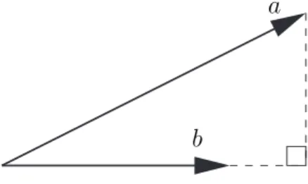
Figure 2.1: The dot product

What if we project a 1-dimensional subspace onto another? The answer is well known; For vectorsaandb, the dot producta·bprojectsaontobresulting in the scalar magnitude of the projection relative to b’s magnitude. This is

(9)

depicted in figure 2.1 for the case wherebis a unit vector.

Scalars can be treated as 0-dimensional subspaces. Thus, the projection of a 1-dimensional subspace onto another results in a 0-dimensional subspace.

2.1

Bivectors

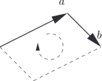
Geometric algebra introduces an operator that is in some ways the opposite of the dot product. It is called the outer product and instead of projecting a vector onto another, it extends a vector along another. The∧(wedge) symbol is used to denote this operator. Given two vectorsa andb, the outer producta∧b is depicted in figure 2.2.

a

b

Figure 2.2: Vector aextended along vectorb

The resulting entity is a 2-dimensional subspace, and we call it a bivector. It has an area equal to the size of the parallelogram spanned byaandband an orientation depicted by the clockwise arc. Note that a bivector has no shape. Using a parallelogram to visualize the area provides an intuitive way of under-standing, but a bivector is just an oriented area, in the same way a vector is just an oriented length.

b

a

Figure 2.3: Vector bextended along vector a

Ifbwere extended alongathe result would be a bivector with the same area but an opposite (ie. counter-clockwise) orientation, as shown in figure 2.3. In mathematical terms; the outer product is anticommutative, which means that:

(10)

With the consequence that:

a∧a= 0 (2.2)

which makes sense if you consider thata∧a=−a∧aand only 0 equals its own negation (0 = -0). The geometrical interpretation is a vector extended along itself. Obviously the resulting bivector will have no area.

Some other interesting properties of the outer product are:

(λa)∧b=λ(a∧b) associative scalar multiplication (2.3)

λ(a∧b) = (a∧b)λ commutative scalar multiplication (2.4)

a∧(b+c) = (a∧b) + (a∧c) distributive over vector addition (2.5) For vectors a, b and c and scalar λ. Drawing a few simple sketches should convince you, otherwise most of the references provide proofs.

2.1.1

The Euclidian Plane

Given ann-dimensional vector athere is no way to visualize it until we see a decomposition onto a basis (e1, e2, ...en). In other words, we expressaas a linear

combination of the basis vectorsei. This allows us to write aas an n-tuple of

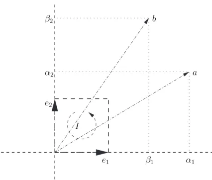
real numbers, e.g. (x, y) in two dimensions, (x, y, z) in three, etcetera. Bivectors are much alike; they can be expressed as linear combinations of basis bivectors. To illustrate, consider two vectorsaandbin the Euclidian PlaneR2_{. Figure} 2.4 depicts the real number decomposition a= (α1, α2) andb = (β1, β2) onto the basis vectorse1and e2.

Written down, this decomposition looks as follows:

a=α1e1+α2e2

b=β1e1+β2e2 The outer product ofaandb becomes:

a∧b= (α1e1+α2e2)∧(β1e1+β2e2) Using (2.5) we may rewrite the above to:

a∧b=(α1e1∧β1e1)+ (α1e1∧β2e2)+ (α2e2∧β1e1)+ (α2e2∧β2e2)

Equation (2.3) and (2.4) tell us we may reorder the scalar multiplications to obtain:

a∧b=(α1β1e1∧e1)+ (α1β2e1∧e2)+ (α2β1e2∧e1)+ (α2β2e2∧e2)

(11)

α

1

I

e

2

e

1

β

1

b

α

2

β

2

a

Figure 2.4: A two dimensional basis

Now, recall equation (2.2) which says that the outer product of a vector with itself equals zero. Thus we are left with:

a∧b=(α1β2e1∧e2)+ (α2β1e2∧e1)

Now take another look at figure 2.4. There, I represents the outer product

e1∧e2. This will be our choice for the basis bivector. Because of (2.1) this means thate2∧e1 =−I. Using this information in the previous equation, we obtain:

a∧b= (α1β2−α2β1)I (2.6) Which is how to calculate the outer product of two vectors a = (α1, α2) and

b= (β1, β2). Thus, in two dimensions, we express bivectors in terms of a basis bivector calledI. In the Euclidian plane we useIto represente12=e1∧e2.

(12)

2.1.2

Three Dimensions

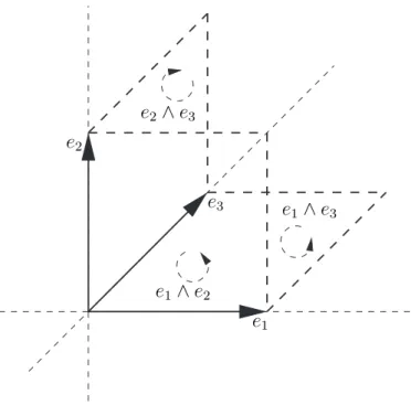
In 3-dimensional spaceR3_{, things become more complicated. Now, the} orthog-onal basis consists of three vectors: e1,e2, ande3. As a result, there are three basis bivectors. These are e1∧e2 = e12, e1∧e3 =e13, and e2∧e3 =e23, as depicted in figure 2.5.

e

1

e

2

e

1

∧

e

2

e

3

e

₁

∧

e

₃

e

2

∧

e

3

Figure 2.5: A 3-dimensional bivector basis

It is worth noticing that the choice between using either eij or eji as a

basis bivector is completely arbitrary. Some people prefer to use{e12, e23, e31} because it is cyclic, but this argument breaks down in four dimensions or higher; e.g. try making{e12, e13, e14, e23, e24, e34}cyclic. I use{e12, e13, e23}because it solves some issues [12] in computational geometric algebra implementations.

The outer product of two vectors will result in a linear combination of the three basis bivectors. I will demonstrate this by using two vectorsaandb:

a=α1e1+α2e2+α3e3

b=β1e1+β2e2+α3e3 The outer producta∧bbecomes:

(13)

Using the same rewrite rules as in the previous section, we may rewrite this to:

a∧b=α1e1∧β1e1+α1e1∧β2e2+α1e1∧β3e3+

α2e2∧β1e1+α2e2∧β2e2+α2e2∧β3e3+

α3e3∧β1e1+α3e3∧β2e2+α3e3∧β3e3 And reordering scalar multiplication:

a∧b=α1β1e1∧e1+α1β2e1∧e2+α1β3e1∧e3+

α2β1e2∧e1+α2β2e2∧e2+α2β3e2∧e3+

α3β1e3∧e1+α3β2e3∧e2+α3β3e3∧e3

Recalling equations (2.1) and (2.2), we have the following rules fori6=j:

ei∧ei= 0 outer product with self is zero

ei∧ej=eij outer product of basis vectors equals basis bivector

ej∧ei=−eij anticommutative

Using this, we can rewrite the above to the following:

a∧b= (α1β2−α2β1)e12+ (α1β3−α3β1)e13+ (α2β3−α3β2)e23 (2.7) which is the outer product of two vectors in 3-dimensional Euclidian space.

For some, this looks remarkably like the definition of the cross product. But they are not the same. The outer product works in all dimensions, whereas the cross product is only defined in three dimensions.1 _{Furthermore, the cross} product calculates a perpendicular subspace instead of a parallel one. Later we will see why this causes problems in certain situations2 _{and how the outer} product solves these.

(14)

2.2

Trivectors

Until now, we have been using the outer product as an operator of two vectors. The outer product extended a 1-dimensional subspace along another to create a 2-dimensional subspace. What if we extend a 2-dimensional subspace along a 1-dimensional one?

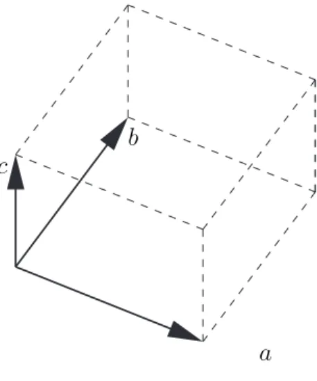
Ifa,bandcare vectors, then what is the result of (a∧b)∧c? Intuition tells us this should result in a 3-dimensional subspace, which is correct and illustrated in figure 2.6.

c

b

a

Figure 2.6: A Trivector

A bivector extended by a third vector results in a directed volume element. We call this a trivector. Note that, like bivectors, a trivector has no shape; only volume and sign. Even though a box helps to understand the nature of trivectors intuitively, it could have been any shape.

In 3-dimensional Euclidian space R3_{, there is one basis trivector equal to}

e1∧e2∧e3 =e123. Sometimes, in Euclidian space, this trivector is called I. We already saw this symbol being used fore12in the Euclidian plane, and we’ll return to it when we discuss pseudo-scalars.

The result of the outer product of three arbitrary vectors results in a scalar multiple of this basis trivector. In 4-dimensional spaceR4_{, there are four basis} trivectors e123, e124, e134, and e234, and consequently an arbitrary trivector will be a linear combination of these four basis trivectors. But what about the Euclidian Plane? Obviously, there can be no 3-dimensional subspaces in a 2-dimensional spaceR2_{. The following informal proof demonstrates why trivectors} do not exist in two dimensions.

We need to show that for arbitrary vectors a, b, and c ∈R2 _{the following} holds:

(15)

Again, we will decompose the vectors onto the basis vectors, using real numbers (α1, α2), (β1, β2), and (γ1, γ2):

a=α1e1+α2e2

b=β1e1+β2e2

c=γ1e1+γ2e2 Using equation (2.6), we may write:

(a∧b)∧c= ((α1β2−α2β1)e1∧e2)∧(γ1e1+γ2e2) We can rewrite this to:

((α1β2−α2β1)e1∧e2)∧(γ1e1) + ((α1β2−α2β1)e1∧e2)∧(γ2e2) Which becomes:

(γ1(α1β2−α2β1)e1∧e2∧e1) + (γ2(α1β2−α2β1)e1∧e2∧e2)

The scalar parts are not really important. Take a good look at the outer product of the basis vectors. We have:

e1∧e2∧e1, and e1∧e2∧e2

Because the outer product is anticommutative (equation (2.1)), we may rewrite the first one:

−e1∧e1∧e2, ande1∧e2∧e2

And using equation (2.2) which says that the outer product of a vector with itself equals zero, we are left with:

−0∧e2, ande1∧0

From here, it does not take much to realize that the outer product of a vector and the null vector results in zero. I’ll come back to a more formal treatment of null vectors later, but for now it should be enough to understand that if we extend a vector by a vector that has no length, we are left with zero area. Thus we conclude thata∧b∧c= 0 inR2_.

(16)

2.3

Blades

So far we have seen scalars, vectors, bivectors and trivectors representing 0-, 1-, 2- and 3-dimensional subspaces respectively. Nothing stops us from generalizing all of the above to allow subspaces with arbitrary dimension.

Therefore, we introduce the term k-blades, wherek refers to the dimension of the subspace the blade spans. The numberkis called the grade of a blade. Scalars are 0-blades, vectors are 1-blades, bivectors are 2-blades, and trivectors are 3-blades. In other words, the grade of a vector is one, and the grade of a trivector is three. In higher dimensional spaces there can be 4-blades, 5-blades, or even higher. As we have shown for n = 2 in the previous section, in an

n-dimensional space then-blade is the blade with the highest grade.

Recall how we expressed vectors as a linear combination of basis vectors and bivectors as a linear combination of basis bivectors. It turns out that every

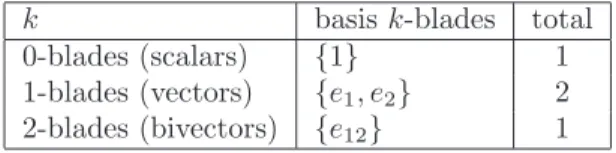
k-blade can be decomposed onto a set of basisk-blades. The following tables contain all the basis blades for subspaces of dimensions 2, 3 and 4.

k basisk-blades total 0-blades (scalars) {1} 1 1-blades (vectors) {e1, e2} 2

2-blades (bivectors) {e12} 1 Figure 2.7: Basis blades in 2 dimensions

k basisk-blades total 0-blades (scalars) {1} 1 1-blades (vectors) {e1, e2, e3} 3

2-blades (bivectors) {e12, e13, e23} 3

3-blades (trivectors) {e123} 1 Figure 2.8: Basis blades in 3 dimensions

k basisk-blades total

0-blades (scalars) {1} 1 1-blades (vectors) {e1, e2, e3, e4} 4

2-blades (bivectors) {e12, e13, e14, e23, e24, e34} 6

3-blades (trivectors) {e123, e124, e134, e234} 4

4-blades {e1234} 1

Figure 2.9: Basis blades in 4 dimensions

Generalizing this; how many basisk-blades are needed in an n-dimensional space to represent arbitraryk-blades? It turns out that the answer lies in the

(17)

binomial coefficient: _µ n k ¶ = n! (n−k)!k!

This is because a basisk-blade is uniquely determined by thekbasis vectors from which it is constructed. There arendifferent basis vectors in total. ¡n_k¢is the number of ways to choosek elements from a set ofn elements and thus it is easily seen that the number of basisk-blades is equal to¡n

k

¢ .

Here are a few examples which you can compare to the tables above. The number of basis bivectors or 2-blades in 3-dimensional space is:

µ 3 2 ¶ = 3! (3−2)!2! = 3

The number of basis trivectors or 3-blades in 3-dimensional space equals: µ 3 3 ¶ = 3! (3−3)!3! = 1

The number of basis bivectors or 2-blades in 4-dimensional space is: µ 4 2 ¶ = 4! (4−2)!2! = 6

(18)

Chapter 3

Geometric Algebra

All spacesRn _{generate a set of basis blades that make up a}_{Geometric Algebra}

of subspaces, denoted byC`n.1 For example, a possible basis forC`2is: { _|{z}1 basis scalar , e1, e2 | {z } basis vectors , _|{z}I basis bivector }

Here, 1 is used to denote the basis 0-blade or scalar-basis. Every element of the geometric algebra C`2 can be expressed as a linear combination of these basis blades. Another example is a basis ofC`3 which could be:

{ _|{z}1 basis scalar , e_|1, e_{z2, e3_} basis vectors , e_|12, e_{z13, e23_} basis bivectors e123 |{z} basis trivector }

The total number of basis blades for an algebra can be calculated by adding the numbers required for all basisk-blades:

n X k=0 µ n k ¶ = 2n (3.1)

The proof relies on some combinatorial mathematics and can be found in many places. You can use the following table to check the formula for a few simple geometric algebras.

C`n basis blades total

C`0 {1} 20= 1

C`1 {1;e1} 21= 2

C`2 {1;e1, e2;e12} 22= 4

C`3 {1;e1, e2, e3;e12, e13, e23;e123} 23= 8

C`4 {1;e1, e2, e3, e4;e12, e13, e14, e23, e24, e34;e123, e124, e134, e234;e1234} 24= 16

1_{The reason we use}_C_`

n is because geometric algebra is based on the theory of Clifford

(19)

3.1

The Geometric Product

Until now we have only used the outer product. If we combine the outer product with the familiar dot product we obtain the geometric product. For arbitrary vectorsa,b the geometric product can be calculated as follows:

ab=a·b+a∧b (3.2)

Wait, how is that possible? The dot product results in a scalar, and the outer product in a bivector. How does one add a scalar to a bivector?

Like complex numbers, we keep the two entities separated. The complex number (3 + 4i) consists of a real and imaginary part. Likewise,ab=a·b+a∧b

consists of a scalar and a bivector part. Such combinations of blades are called multivectors.

3.2

Multivectors

A multivector is a linear combination of differentk-blades. InR2_{it will contain} a scalar part, a vector part and a bivector part:

α1 |{z} scalar part + α_|2e1_{z+α3e2_} vector part + _|{z}α4I bivector part

Whereαi are real numbers, e.g. the components of the multivector. Note that

αi can be zero, which means that blades are multivectors as well. For example,

ifa1 anda4 are zero, we have a vector or 1-blade.

InR2 _{we need 2}2 _{= 4 real numbers to denote a full multivector. A} multi-vector inR3_{can be defined with 2}3_{= 8 real numbers and will look like this:}

α1 |{z} scalar part + _|α2e1+α_{z3e2+α4e3_} vector part +_|α5e12+α6_{ze13+α7e23_} bivector part + α_{| {z }}8e123 trivector part

In the same way, a multivector inR4_{will have 2}4_{= 16 components.}

Unfortunately, multivectors can’t be visualized easily. Vectors, bivectors and trivectors have intuitive visualizations in 2- and 3-dimensional space. Multivec-tors lack this way of thinking, because we have no way to visualize a scalar added to an area. However, we get something much more powerful than easy visualization. A multivector, as a linear combination of subspaces, turns out to be extremely expressive, and can be used to convey many different concepts in geometry.

(20)

3.3

The Geometric Product Continued

The generalized geometric product is an operator for multivectors. It has the following properties:

(AB)C=A(BC) associativity (3.3)

λA=Aλ commutative scalar multiplication (3.4)

A(B+C) =AB+AC distributive over addition (3.5) For arbitrary multivectors A, B and C, and scalar λ. Proofs for the other properties are beyond the scope of this paper. They are not difficult per se, but it is mostly formal algebra even though all of the above intuitively feel right already. The interested reader should pick up some of the references for more information.

Note that the geometric product is, in general, not commutative:

AB6=BA

Nor is it anticommutative. This is a direct consequence of the fact that the anticommutative outer product and the commutative dot product are both part of the geometric product.

We have seen the geometric product for vectors using the dot product and the outer product. However, since the dot product is only defined for vectors, and the outer product only for blades, we need something different for multivectors.

Consider two arbitrary multivectorsAandB fromC`2.

A=α1+α2e1+α3e2+α4I

B=β1+β2e1+β3e2+β4I Multiplying A and B using the geometric product, we get:

AB= (α1+α2e1+α3e2+α4I)B Using equation (3.5) we may rewrite this to:

AB=α1B+α2e1B+α3e2B+α4IB Now writing out B:

AB= (α1 (β1+β2e1+β3e2+β4I)) + (α2e1(β1+β2e1+β3e2+β4I)) + (α3e2(β1+β2e1+β3e2+β4I)) + (α4I (β1+β2e1+β3e2+β4I)) And this can be rewritten to:

AB=α1β1 +α1β2e1 +α1β3e2 +α1β4I +α2e1β1+α2e1β2e1+α2e1β3e2+α2e1β4I +α3e2β1+α3e2β2e1+α3e2β3e2+α3e2β4I +α4Iβ1 +α4Iβ2e1 +α4Iβ3e2 +α4Iβ4I

(21)

And in the same way as we did when we wrote out the outer product, we may reorder the scalar multiplications (3.4) to obtain:

AB=α1β1 +α1β2e1 +α1β3e2 +α1β4I (3.6) +α2β1e1+α2β2e1e1+α2β3e1e2+α2β4e1I

+α3β1e2+α3β2e2e1+α3β3e2e2+α3β4e2I +α4β1I +α4β2Ie1 +α4β3Ie2 +α4β4II

This looks like a monster of a calculation at first. But if you study it for a while, you will notice that it is fairly structured. The resulting equation demon-strates that we can express the geometric product of arbitrary multivectors as a linear combination of geometric products of basis blades.

So what we need, is to understand how to calculate geometric products of basis blades. Let’s look at a few different combinations. For example, using equation (3.2) we can write:

e1e1=e1·e1+e1∧e1

But remember from equation (2.2) thata∧a= 0 because it has no area. Also, the dot product of a vector with itself is equal to its squared magnitude. If we choose the magnitude of the basis vectorse1,e2, etc. to be 1, we may simplify the above to:

e1e1=e1·e1+e1∧e1 =e1·e1+0

= 1 +0

= 1 Another example is, again inC`2:

e1e2=e1·e2+e1∧e2

Now remember that e1 is perpendicular to e2 so the dot product e1·e2 = 0. This leaves us with:

e1e2=e1·e2+e1∧e2 = 0 +e1∧e2

= 0 +I

=I

A more complicated example involves the geometric product of e1 and I. The previous example showed us thatI=e12is equal to e1e2. We can use this

(22)

and equation (3.3) to write: e1I=e1e12 =e1(e1e2) = (e1e1)e2 = 1e2 =e2

You might begin to see a pattern. Because the basis blades are perpendicular, the dot and outer product have trivial results. We use this to simplify the result of a geometric product with a few rules.

1. Basis blades with grades higher than one (bivectors, trivectors, 4-blades, etc.) can be written as an outer product of perpendicular vectors. Because of this, their dot product equals zero, and consequently, we can write them as a geometric product of vectors. For example, in some high dimensional space, we could write:

e12849=e1∧e2∧e8∧e4∧e9=e1e2e8e4e9

2. Equation (2.1) allows us to swap the order of two non-equal basis vectors if we negate the result. This means that we can write:

e1e2e3=−e2e1e3=e2e3e1=−e3e2e1

3. Whenever a basis vector appears next to itself, it annihilates itself, because the geometric product of a basis vector with itself equals one.

eiei = 1 (3.7)

Example:

e112334=e24

Using these three rules we are able to simplify any geometric product of basis blades. Take the following example:

e1e23e31e2= e1e2e3e3e1e2 using rule one = e1e2e1e2 using rule three =−e1e1e2e2 using rule two

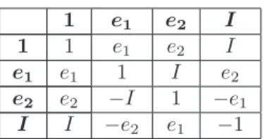
= −1 using rule three twice

(3.8) We can now create a so-called multiplication table which lists all the combi-nations of geometric products of basis blades. ForC`2 it would look like figure 3.1.

(23)

1 e1 e2 I

1 1 e1 e2 I

e1 e1 1 I e2

e2 e2 −I 1 −e1

I I −e2 e1 −1

Figure 3.1: Multiplication Table for basis blades in C`2

According to this table, the multiplication ofIandIshould equal−1, which can be calculated as follows:

I2₌ _e

12e12 by definition

= e1e2e1e2 using rule one =−e2e1e1e2 using rule two

=−e2e2 using rule three

=−1 using rule three

Now that we have the required knowledge on geometric products of basis blades, we can return to the geometric product of arbitrary blades. Here’s equation (3.6) repeated for convenience:

AB=α1β1 +α1β2e1 +α1β3e2 +α1β4I +α2β1e1+α2β2e1e1+α2β3e1e2+α2β4e1I +α3β1e2+α3β2e2e1+α3β3e2e2+α3β4e2I +α4β1I +α4β2Ie1 +α4β3Ie2 +α4β4II

We can simply look up the geometric product of basis blades in the multiplica-tion table, and substitute the results:

AB=α1β1 +α1β2e1+α1β3e2+α1β4I +α2β1e1+α2β2 +α2β3I +α2β4e2 +α3β1e2−α3β2I +α3β3 −α3β4e1 +α4β1I −α4β2e2+α4β3e1−α4β4 Now the last step is to group the basis-blades together.

AB= (α1β1+α2β2+α3β3−α4β4) (3.9) + (α4β3−α3β4+α1β2+α2β1)e1

+ (α1β3−α4β2+α2β4+α3β1)e2 + (α4β1+α1β4+α2β3−α3β2)I

(24)

That is to say; so far I have only showed you how the geometric product works inC`2. It is trivial to extend the same methods to C`3 or higher. The same three simplification rules apply. Figure 3.2 contains the multiplication table forC`3. 1 e1 e2 e3 e12 e13 e23 e123 1 1 e1 e2 e3 e12 e13 e23 e123 e1 e1 1 e12 e13 e2 e3 e123 e23 e2 e2 −e12 1 e23 −e1 −e123 e3 −e13 e3 e3 −e13 −e23 1 e123 −e1 −e2 e12 e12 e12 −e2 e1 e123 −1 −e23 e13 −e3 e13 e13 −e3 −e123 e1 e23 −1 −e12 e2 e23 e23 e123 −e3 e2 −e13 e12 −1 −e1 e123 e123 e23 −e13 e12 −e3 e2 −e1 −1

Figure 3.2: Multiplication Table for basis blades in C`3

3.4

The Dot and Outer Product revisited

We defined the geometric product for vectors as a combination of the dot and outer product:

ab=a·b+a∧b

We can rewrite these equations to express the dot product and outer product in terms of the geometric product:

a∧b= 1

2(ab−ba) (3.10)

a·b= 1

2(ab+ba) (3.11)

To illustrate, let us prove (3.10). Let’s take two multivectors A and B∈ C`2 for which the scalar and bivector parts are zero, e.g. two vectors. Using equation (3.9) and taking into account that α1 =β1 =α4 =β4 = 0 we can write AB andBAas:

AB= (α2β2+α3β3) (3.12)

+ (α2β3−α3β2)I

BA= (β2α2+β3α3) (3.13)

(25)

Using these in equation (3.10) we get: AB z }| { ((α2β2+α3β3) + (α2β3−α3β2)I)− BA z }| { ((β2α2+β3α3) + (β2α3−β3α2)I) 2 Reordering we get: ScalarP art z }| { (α2β2+α3β3)−(β2α2+β3α3) + BivectorP art z }| { (α2β3−α3β2)I−(β2α3−β3α2)I 2

Notice the scalar part results in zero, which leaves us with: (α2β3−α3β2)I−(β2α3−β3α2)I

2 Subtracting the two bivectors we get:

(α2β3−α3β2−β2α3+β3α2)I 2

This may be rewritten as:

(2α2β3−2α3β2)I 2

And now dividing by 2 we obtain:

A∧B= (α2β3−α3β2)I

for multivectorsAandBwith zero scalar and bivector part. Compare this with equation (2.6) that defines the outer product for two vectorsa and b. If you remember that the vector part of a multivector∈ C`2is in the second and third component, you will realize that these equations are the same.

Note that (3.10) and (3.11) only hold for vectors. The inner and outer product of higher order blades is more complicated, not to mention the inner and outer product for multivectors. Yet, let us try to see what they could mean.

3.5

The Inner Product

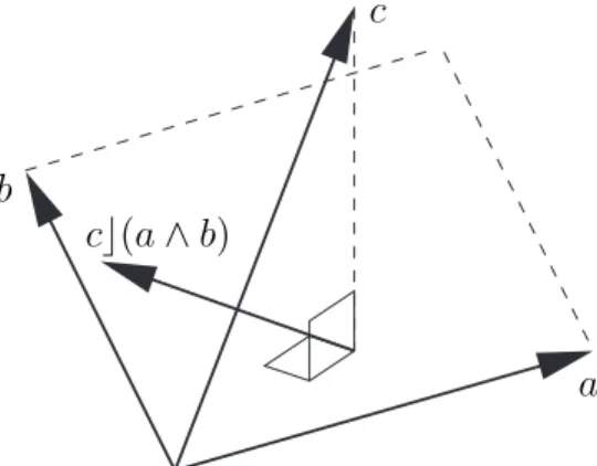
I informally demonstrated what the outer product of a vector and a bivector looks like when I introduced trivectors. What about the dot product? What could the dot product of a vector and a bivector look like? Figure 3.3 depicts the result.

Notice how the inner product is the vector perpendicular to the actual pro-jection. In more general terms, it is thecomplement (within the subspace ofB)

(26)

c

(

a

∧

b

)

a

b

c

Figure 3.3: The dot product of a bivector and a vector

Unfortunately, there is not just one definition of the inner product. There are several versions floating around, their usefulness depending on the problem area. They are not fundamentally different however, and all of them can be expressed in terms of the others. In fact, one could say that the flexibility of the different inner products is one of the strengths of geometric algebra. Unfortunately, this does not really help those trying to learn geometric algebra, as it can be overwhelming and confusing.

The default and best known inner product [8] is very useful in Euclidian me-chanics, whereas thecontraction inner product [2], also known as the Lounesto inner product, is more useful in computer science. Other inner products in-clude the semi-symmetric or semi-commutative inner product, also known as the Hestenes inner product, the modified Hestenes or (fat)dot product and the forced Euclidean contractive inner product. [13] [5]

Obviously, because of our interest for computer science, we are most inter-ested in the contraction inner product. We will use thec symbol to denote a contraction. It may seem a bit weird at first, but it will turn out to be very useful. Luckily, for two vectors it works exactly as the traditional inner product or dot product. For different blades, it is defined as follows [2]:

scalars αcβ=αβ (3.14)

vector and scalar acβ= 0 (3.15)

scalar and vector αcb=αb (3.16)

vectors acb=a·b (the usual dot product) (3.17) vector, multivector ac(b∧C) = (acb)∧C−b∧(acC) (3.18) distribution (A∧B)cC=Ac(BcC) (3.19) Try to understand how the above provides a recursive definition of the con-traction operator. There are the basic rules for vectors and scalars, and there is (3.18) for the contraction between a vector and the outer product of a vector and

(27)

a multivector. Because linearity holds over the contraction, we can decompose contractions with multivectors into contractions with blades. Now, remember that any bladeD with gradencan be written as the outer product of a vector

b and a blade C with grade n−1. This means that the contraction acD can be written as ac(b∧C) and consequently as (acb)∧C−b∧(acC) according to (3.18). We know how to calculateacb by definition, and we can recursively solveacC until the grade of C is equal to 1, which reduces it to a contraction of two vectors.

Obviously, this is not a very efficient way of calculating the inner product. Fortunately, the inner product can be expressed in terms of the geometric prod-uct (and vice versa as we’ve done before), which allows for fast calculations. [12]

I will return to the inner product when I talk about grades some more in the tools chapter. In the chapter on applications we will see where and how the contraction product is useful. From now on, whenever I refer to the inner product I mean any of the generalized inner products. If I need the contraction, I will mention it explicitly. I will allow myself to be sloppy, and continue to use the· andcsymbol interchangeably.

3.6

Inner, Outer and Geometric

We saw in equation (3.2) that the geometric product for vectors could be defined in terms of the dot (inner) and outer product. What if we use (3.10) and (3.11) combined: 1 2(ab+ba) + 1 2(ab−ba) = (ab+ba) + (ab−ba) 2 =(ab+ba+ab−ba) 2 =2ab 2 =ab

This demonstrates the two possible approaches to introduce geometric alge-bra. Some books [7] give an abstract definition of the geometric product, by means of a few axioms, and derive the inner and outer product from it. Other material [8] starts with the inner and outer product and demonstrates how the geometric product follows from them.

You may prefer one over the other, but ultimately it is the way the geometric product, the inner product and the outer product work together that gives geometric algebra its strength. For two vectorsaandbwe have:

(28)

wedge of two collinear vectors is zero. If the two vectors are neither collinear nor orthogonal the geometric product is able to express their relationship as ‘something in between’.

(29)

Chapter 4

Tools

Strictly speaking, all we need is an algebra of multivectors with the geometric product as its operator. Nevertheless, this chapter introduces some more defi-nitions and operators that will be of great use in many applications. If you are tired of all this theory, I suggest you skip over this section and start with some of the applications. If you encounter unfamiliar concepts, you can refer to this chapter.

4.1

Grades

I briefly talked about grades in the chapter on subspaces. The grade of a blade is the dimension of the subspace it represents. Thus multivectors have combinations of grades, as they are linear combinations of blades. We denote the blade-part with grade s of a multivector A using hAis. For multivector

A= (4,8,5,6,2,4,9,3)∈ C`3 we have:

hAi0= 4 scalar part

hAi1= (8,5,6) vector part hAi2= (2,4,9) bivector part

hAi3= 3 trivector part

Any multivectorAinC`ncan be denoted as a sum of blades, like we already

did informally:

n

X

k=0

hAik=hAi0+hAi1+. . .+hAin

Using this notation I can demonstrate what the inner and outer product mean for grades. For two vectors a and b the inner product a·b results in a

(30)

In figure 3.3 we saw that a vectora projected onto a bivector B resulted in a vector. Here, we’ll be using the contraction product. So, in other words the contraction product of a 2-blade and a 1-blade results in a 1-blade. Using a multivector notation:

hai1chBi2=haBi2−1

Generalizing this for bladesAandB with gradesandtrespectively: hAischBit=hABiu where u=

½

s > t, 0

s≤t, t - s

We might say that the contraction inner product is a ’grade-lowering’ operation. And, of course, the outer product is its opposite as a grade-increasing op-eration. Recall that for two 1-blades or vectors the outer product resulted in a 2-blade or bivector:

hai1∧ hbi1=habi2

The outer product between a 2-blade and a 1-blade results in a 2 + 1 = 3-blade or trivector. Generalizing we get for two bladesAandB with gradesandt:

hAis∧ hBit=hABis+t

Note that A and B have to be blades. These equations do not hold when they are arbitrary multivectors.

4.2

The Inverse

Most multivectors have a left inverse satisfyingA−1L_A_{= 1 and a right inverse}

satisfying AA−1R _{= 1. We can use these inverses to divide a multivector by}

another. Recall that the geometric product is not commutative therefore the left and right inverse may or may not be equal. This means that the A

B notation

is ambiguous since it can mean bothB−1LAandAB−1R.

Unfortunately calculating the inverse of a geometric product is not trivial, much like calculating inverses of matrices is complicated for all but a few special cases.

Luckily there is an important set of multivectors for which calculating the inverse is very straightforward. These are called theversors and they have the property that they are a geometric product of vectors. A multivector A is a versor if it can be written as:

A=v1v2v3...vk

wherev1...vk are vectors, i.e. 1-blades. As a fortunate consequence, all blades

are versors too.1 _{For a versor} _A_{we define its}_reverse_{, using the}_†_{symbol, as:}

A†₌_v

kvk−1...v2v1 (4.1)

1_{Remember that we use vectors to create subspaces of higher dimension, using the outer}

(31)

This means that, because of equation (2.1), the reverse of a blade is only a possible sign change. Remember that each swap of indices in the product produces a sign change, thus ifkis uneven the reverste of A is equal to itself, and if it’s uneven the reverse ofA is the−A. Note that this does not apply to versors in general.

The left and right inverse of a versor are the same and can be calculated as follows:

A−1₌ A†

A†_A (4.2)

To understand this, we have to start by realizing that the denominator is always a scalar because:

A†A=v1v2...vk−1vkvkvk−1...v2v1=|v1|2|v2|2...|vk−1|2|vk|2

And since a scalar divided by itself equals one, this means that:

A−1A= A †

A†_AA=

A†_A

A†_A = 1

Furthermore it also proves that the left and right inverse are the same. Division by a scalar α is multiplication by 1/α, which is, according to equation (3.3) commutative, proving that the left and right inverses of a versor are indeed equal.

This means that for a versorA, we haveA−1L ₌_A−1R₌_A−1_{and therefore}

the following:

A−1L_A₌_AA−1R₌_A−1_A₌_AA−1_{= 1}

It is important to notice that in the case of vectors, the scalar represents the squared magnitude of the vector. As a consequence, the inverse of a unit vector is equal to itself.

Not many people are comfortable with the idea of division by vectors, bivec-tors, or multivectors. They are only accustomed to division by scalars. But if we have a geometric product and a definition for the inverse, nothing stops us from division. Later we will see that this is extremely useful.

4.3

Pseudoscalars

In equation (2.3) we saw how to calculate the number of basis blades for a given grade. From this it follows that every geometric algebra has only one basis 0-blade or basis-scalar, independent of the dimension of the algebra:

µ n 0 ¶ = n! (n−0)!0! = n! n! = 1

More interesting is the basis blade with the highest dimension. For a geometric algebraC`n the number of blades with dimension n is:

(32)

In C`2 this was e1e2 = I as shown in figure 2.4. In C`3 this is the trivector

e1e2e3=e123.

In general every geometric algebra has a single basis blade of highest dimen-sion. This is called the pseudoscalar.

4.4

The Dual

Traditional linear algebra uses normal vectors to represent planes. Geometric algebra introduces bivectors which can be used for the same purpose. By using the pseudoscalar we can get an understanding of the relationship between the two representations.

The dualA∗ _{of a multivector A is defined as follows:}

A∗₌_AI−1 _(4.3)

whereIrepresents the pseudoscalar of the geometric algebra that is being used. The pseudoscalar is a blade (the blade with highest grade) and therefore its left and right inverse are the same, and hence the above formula is not ambiguous. Let us consider a simple example in C`3, calculating the dual of the basis bivectore12. The pseudoscalar ise123. Pseudoscalars are blades and thus ver-sors. You can check yourself that its inverse ise3e2e1. We’ll use this to calculate the dual ofe12: e∗ 12=e12e3e2e1 =e1e2e3e2e1 =−e1e3e2e2e1 =−e1e3e1 =e1e1e3 =e3 (4.4) Thus, the dual is basis vector e3, which is exactly the normal vector of basis bivector e12. In fact, this is true for all bivectors. If we have two arbitrary vectorsaandb ∈ C`3:

a=α1e1+α2e2+α3e3

b=β1e1+β2e2+β3e3 According to equation (2.7) their outer product is:

(33)

And its dual (a∧b)∗ _becomes: (a∧b)∗₌₍_a_∧_b₎_e−1 123 =(a∧b)e3e2e1 =((α1β2−α2β1)e12+ (α1β3−α3β1)e13+ (α2β3−α3β2)e23)e3e2e1 =(α1β2−α2β1)e12e3e2e1+ (α1β3−α3β1)e13e3e2e1+ (α2β3−α3β2)e23e3e2e1 =(α1β2−α2β1)e1e2e3e2e1+ (α1β3−α3β1)e1e3e3e2e1+ (α2β3−α3β2)e2e3e3e2e1 =(α1β2−α2β1)e3−(α1β3−α3β1)e2+ (α2β3−α3β2)e1 =(α2β3−α3β2)e1+ (α3β1−α1β3)e2+ (α1β2−α2β1)e3 (4.5) Which is exactly the traditional cross product. We conclude that in three di-mensions, the dual of a bivector is its normal. The dual can be used to convert between bivector and normal representations. But the dual is even more, be-cause it is defined for any multivector.

4.5

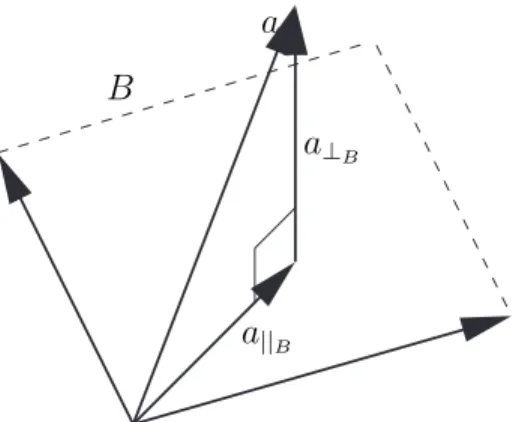
Projection and Rejection

If we have a vector a and bivector B we can decompose a in two parts. One parta||B that is collinear with B. We call this theprojection ofaontoB. The

other part isa⊥B, and orthogonal to B. We call this the rejection

2 _of_a _from

B. Mathematically:

a=a||B+a⊥B (4.6)

This is depicted in figure 4.1. Such a decomposition turns out to be very useful and I will demonstrate how to calculate it.

First, equation (3.2) says that the geometric product of two vectors is equal to the sum of the inner and outer product. There is a generalization of this saying that for arbitrary vectoraandk-bladeB the geometric product is:

(34)

a

B

a

||B

a

⊥B

Figure 4.1: Projection and rejection of vectorain bivectorB

Note thatahas to be a vector, andBa blade of any grade. That is, this doesn’t hold for multivectors in general. Proofs can be found in the references. [14] [8] Using (4.7) we can calculate the decomposition (4.6) of any vectoraonto a bivectorB. By definition, the inner and outer product of respectively orthogonal and collinear blades are zero. In other words, the inner product of a vector orthogonal to a bivector is zero:

a⊥B·B= 0 (4.8)

Likewise the outer product of a vector collinear with a bivector is zero:

a||B∧B = 0 (4.9)

Let’s see what happens if we multiply the orthogonal part of vector a with bivector B: a⊥BB=a⊥B·B+a⊥B∧B =a⊥B∧B using equation (4.8) =a⊥B∧B+a||B∧B equation (4.9) = (a⊥B+a||B)∧B equation (2.5) =a∧B equation (4.6)

Thus, the perpendicular part of vector a times bivector B is equal to the outer product of a and B. Now all we need to do is divide both sides of the equation byB to obtain the perpendicular part ofa:

a⊥BB=a∧B

a⊥BBB

−1_{= (}_a_∧_B₎_B−1

a⊥B = (a∧B)B

(35)

Notice that there is no ambiguity in using the inverse because B is a blade or versor, and its left and right inverses are therefore the same. The conclusion is:

a⊥B = (a∧B)B

−1 _(4.10)

Calculating the collinear part of vectorafollows similar steps:

a||BB=a||B·B+a||B∧B

=a||B·B

=a||B·B+a⊥B·B

= (a⊥B+a||B)·B

=a·B

Again multiply both sides with the inverse bivector:

a||BBB

−1_{= (}_a_·_B₎_B−1 To conclude:

a||B = (a·B)B

−1 _(4.11)

Using these definitions, we can now confirm thata||B+a⊥B =a

a||B+a⊥B = (a∧B)B

−1_{+ (}_a_·_B₎_B−1 _{equation (4.11) and (4.10)}

= (a∧B+a·B)B−1 _{equation (3.3)}

=aBB−1 _{equation (4.7)}

(36)

4.6

Reflections

Armed with a way of decomposing blades in orthogonal and collinear parts we can take a look at reflections. We will get ahead of ourselves and take a specific look at the geometric algebra of the Euclidian space R3 _{denoted with} C`3. Suppose we have a bivector U. Its dual U∗ _{will be the normal vector} _u_. What if we multiply a vectora with vectoru, projecting and rejecting a onto

U at the same time:

ua=u(a||U +a⊥U)

=ua||U +ua⊥U

Using (3.2) we write it in full:

ua= (u·a||U +u∧a||U) + (u·a⊥U +u∧a⊥U)

Note that (because u is the normal of U) the vectors a||U and u are

perpen-dicular. This means that the inner product a||U ·uequals zero. Likewise, the

vectors a⊥U and u are collinear. This means that the outer product a||U ∧u

equals zero. Removing these two 0 terms:

ua=u∧a||U +u·a⊥U

=u·a⊥U +u∧a||U

Recall that the inner product between two vectors is commutative, and the outer product is anticommutative, so we can write:

ua=a⊥U ·u−a||U ∧u

We can now insert those 0-terms back in (putting in the form of equation (3.2)):

ua= (a⊥U ·u+a⊥U ∧u)−(a||U·u+a||U∧u)

Writing it as a geometric product now:

ua=a||Uu−a⊥Uu

= (a||U−a⊥U)u

Meaning that:

−ua=−(a||U −a⊥U)u

= (a⊥U −a||U)u

Notice how we changed the addition of the perpendicular part into a subtraction by multiplying with −u. Now, if we add a multiplication with the inverse we obtain the following, depicted in figure 4.2:

−uau−1₌₋_u₍_a ||U +a⊥U)u −1 = (a||U−a⊥U)uu −1 =a||U −a⊥U

(37)

a

||U

−

a

⊥U

=

−

uau

−1

a

||U

a

⊥U

a

U

u

Figure 4.2: Reflection

In general, if we sandwich a vector a in between another vector −u and its inverseu−1_{, we obtain a reflection in the dual}_u∗_.

Note that in many practical cases uwill be a unit vector, which means its inverse isuitself. Thus the reflection of a vector ain a plane with unit-normal

u is simply −uau. Later, we will see that reflections are not only useful by themselves, but combined they allow us to do rotations.

(38)

4.7

The Meet

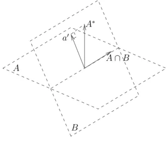
The meet operator is an operator between two arbitrary bladesA and B and defined as follows:

A∩B=A∗_·_B

In other words, the meetA∩Bis the inner product of the dual ofAwithB. It is no coincidence that the∩symbol is used to denote the meet. The result of a meet represents the smallest common subspaces of bladesA andB. Let’s see, in an informal way, what the meet operator does for two bivectors. Looking at figure 4.3 we see two bivectorsAandB.

A

∩

B

A

∗

a

0

B

A

Figure 4.3: The Meet

In this figure, the dual of bivectorAwill be the normal vectorA∗_{. Then, as} we’ve already seen, the inner product of this vector with bivectorB will create the vector perpendicular to the projected vectora0_{. This is exactly the vector} that lies on the intersection of the two bivectors.

A more formal proof of the above, or even the full proof that the meet operator represents the smallest common subspace of any two blades, is far from trivial and beyond this paper. Here, I just want to demonstrate that there is a meet operator, and that it is easily defined using the dual and the inner product. We will be using the meet operator later when we talk about intersections between primitives.

(39)

Chapter 5

Applications

Up until now I haven’t focused on the practical value of geometric algebra. With an understanding of the fundamentals, we can start applying the theory to real world domains. This is where geometric algebra reveals its power, but also its difficulty.

Geometric algebra supplies us with an arithmetic of subspaces, but it is up to us to interpret each subspace and operation and relate it to some real-life concept. This chapter will demonstrate how different geometric algebras com-bined with different interpretations can be used to explain traditional geometric relations.

5.1

The Euclidian Plane

For an easy start, we’ll consider the two dimensional Euclidian Plane to learn about some of the things its geometric algebraC`2has to offer.

5.1.1

Complex Numbers

If you recall the geometric algebra of the Euclidian Plane, you might remember we usedIto denote the basis bivector. Then, in table 3.1 we saw thatI2₌_−1. Thus, we might say:

I=√−1

Suppose we interpret a multivector with a scalar and bivector blade as a complex number. The scalar corresponds to the real part, and the bivector to the imaginary part. Thus, we can interpret a multivector (α1, α2, α3, α4) from C`2as a complex numberα1+iα4 as long asα2andα3 are zero.

Not surprisingly, multivector addition and subtraction corresponds directly with complex number addition and subtraction. But even more so, the geometric

(40)

Recall equation (3.9); the full geometric product of multivectorsA= (α1, α2, α3, α4) andB= (β1, β2, β3, β4), repeated here:

AB= ((α1β1) + (α2β2) + (α3β3)−(α4β4)) + ((α4β3)−(α3β4) + (α1β2) + (α2β1))e1 + ((α1β3)−(α4β2) + (α2β4) + (α3β1))e2 + ((α4β1) + (α1β4) + (α2β3)−(α3β2))I

If A and B are complex numbers, α2, α3, β2 and β3 will equal zero. Thus we can discard those parts to obtain:

AB= ((α1β1)−(α4β4)) + ((α4β1) + (α1β4))I

Withα1andβ1 being the real parts, andα4 andβ4being the imaginary parts, this is exactly a complex number multiplication.

5.1.2

Rotations

I will discuss rotations in two dimensions very briefly. When we return to rotations in three dimensions I will introduce the more general dimension-free theory and give several longer and more formal proofs.

If we want to rotate a vector a= α2e1+α3e2 over an angle θ into vector

a0₌_α0

2e1+α03e2, we can employ the following well known formulas:

α0

2= cos(θ)α2−sin(θ)α3 (5.1)

α03= sin(θ)α2+ cos(θ)α3 (5.2) Or, more commonly we employ the matrix formulaa0 ₌_{M a}_where_M _is:

·

cos(θ) −sin(θ) sin(θ) cos(θ)

¸

Returning to geometric algebra, let us see what happens if we multiply vector

awith a complex numberB=β1+β4Ito obtain:

a00=aB = (α2e1+α3e2)(β1+β4I) =α2e1(β1+β4I) +α3e2(β1+β4I) =α2e1β1+α2e1β4I+α3e2β1+α3e2β4I =β1α2e1+β4α2e1I+β1α3e2+β4α3e2I =β1α2e1+β4α2e1e1e2+β1α3e2+β4α3e2e1e2 =β1α2e1+β4α2e2+β1α3e2−β4α3e1 = (β1α2−β4α3)e1+ (β4α2+β1α3)e2

(41)

Thus we see that the geometric product of a complex number and a vector results in a vector with components:

α00

2 =β1α2+β4α3

α003 =β4α2−β1α3

(5.3) Compare this with equations (5.1) and (5.2). If we takeβ1= cos(θ) and a

β4= sin(θ) we can use complex numbers to do rotations, because then:

α02= cos(θ)α2−sin(θ)α3=β1α2−β4α3=α002

α0

3= sin(θ)α2+ cos(θ)α3=β4α2+β1α3=α003

At this point we no longer talk about complex numbers but we call B a spinor. In general, spinors are n-dimensional rotators, and in C`2 they are represented by a linear combination of a scalar plus a bivector.

Equation (3.2) says that the geometric product of two vectors is a scalar plus a bivector. So let’s find apandqthat generate B:

B =β1+β4I=p·q+p∧q=pq

Traditional vector algebra tells us that the angle between two unit vectors can be expressed using the dot product, i.e. p·q= cos(θ). It also tells us that the magnitude of the cross product of two unit vectors is equal to the sine of the same angle,|p×q|= sin(θ).

I already demonstrated that the cross product is related to the outer product through the dual. In fact, it turns out that the outer product between two unit vectors is exactly the sine of their angle times the basis bivector I. In other words:

p·q= cos(θ)

p∧q= sin(θ)I

A thorough proof can be found in Hestenes’s New Foundations For Classical Mechanics [8]. The consequence is that, because of equation (3.2), for unit vectorspandq:

pq= cos(θ) + sin(θ)I

withθbeing the angle between the two vectors.

Concluding, a spinor in C`2 is a scalar plus a bivector. Its components correspond directly to the sine and cosine of the angle. The geometric product of two unit vectors generates a spinor.

We can derive this in a similar way by creating the following identity:

(42)

Which is not ambiguous, and can also be written as:

pq−1₌_a0_a−1

Basically, this says that “whatpis toq, isa0 _to _a_{.” We can rewrite this to:}

a0₌_pq−1_a

But the inverse of a unit vector is equal to itself, and thus:

a0₌ _pq |{z}

spinor

a

If the spinorpqrepresents a clockwise rotation, thenqprepresents a counter-clockwise rotation. This is thanks to the fact that the geometric product is not commutative or anticommutative. As a result it can convey more information removing much of the ambiguities of traditional methods where certain repre-sentations can only identify the rotation over the smallest angle.

It’s interesting to look at the rotation over 180 degrees. We can do it by constructing a spinor out of the basis vectore1and its negation−e1. Obviously there is a 180 degree angle between them. If we multiply them (see table 3.1 for a refresher), we get:

e1(−e1) =−(e1e1) =−1

which makes sense because a rotation over 180 degrees reverses the signs. But this becomes more interesting if we do it through two successive rotations over 90 degrees. A rotation by 90 degrees is a multiplication with the basis bivector

I. As an example, consider the following geometric products between the basis bladese1, e2 and I, taken directly from the multiplication table for C`2 as in figure 3.1.

Ie1=−e2

Ie2=e1

I(−e1) =e2

I(−e2) =−e1 Now doing two successive rotations:

I2_e <