Accepted Manuscript
Title: Asynchronous Accelerating Multi-leader Salp Chains for Feature Selection
Author: Ibrahim Aljarah Majdi Mafarja Ali Asghar Heidari Hossam Faris Yong Zhang Seyedali Mirjalili
PII: S1568-4946(18)30428-9
DOI: https://doi.org/doi:10.1016/j.asoc.2018.07.040
Reference: ASOC 5008
To appear in: Applied Soft Computing
Please cite this article as: Ibrahim Aljarah, Majdi Mafarja, Ali Asghar Heidari, Hossam Faris, Yong Zhang, Seyedali Mirjalili, Asynchronous Accelerating Multi-leader Salp Chains for Feature Selection,<![CDATA[Applied Soft Computing Journal]]>(2018), https://doi.org/10.1016/j.asoc.2018.07.040
This is a PDF file of an unedited manuscript that has been accepted for publication. As a service to our customers we are providing this early version of the manuscript. The manuscript will undergo copyediting, typesetting, and review of the resulting proof before it is published in its final form. Please note that during the production process errors may be discovered which could affect the content, and all legal disclaimers that apply to the journal pertain.
Accepted Manuscript
Highlights:
A novel feature selection approach based on binary Salp Swarm Algorithm (SSA) is proposed.
Asynchronous updating rules and leadership structure were used to adapt the salps’ positions.
The number of leaders in the social organization of the artificial salp chain is well studied.
The salp chain is divided into several sub-chains.
The salps in each sub-chain can follow a different strategy to adaptively update their locations. *Highlights (for review)
Accepted Manuscript
Accepted Manuscript
Asynchronous Accelerating Multi-leader Salp Chains for
Feature Selection
Ibrahim Aljaraha, Majdi Mafarjab, Ali Asghar Heidaric, Hossam Farisa, Yong Zhangd,
Seyedali Mirjalilie
aKing Abdullah II School for Information Technology, The University of Jordan, Amman, Jordan
{hossam.faris,i.aljarah}@ju.edu.jo
bDepartment of Computer Science, Birzeit University, Birzeit, Palestine
[email protected], [email protected]
cSchool of Surveying and Geospatial Engineering, University of Tehran, Tehran, Iran
dSchool of Information and Electronic Engineering, China University of Mining and Technology, Xunzhou,
221116, China [email protected]
eInstitute of Integrated and Intelligent Systems, Griffith University, Nathan, Brisbane, QLD 4111, Australia
Abstract
Feature selection is an imperative preprocessing step that can positively affect the perfor-mance of data mining techniques. Searching for the optimal feature subset amongst an unabridged dataset is a challenging problem, especially for large-scale datasets. In this re-search, a binary Salp Swarm Algorithm (SSA) with asynchronous updating rules and a new leadership structure is proposed. To set the best leadership structure, several extensive experiments are performed to determine the most effective number of leaders in the social organization of the artificial salp chain. Inspired from the behaviour of a termite colony (TC) in dividing the termites into four types, the salp chain is then divided into several sub-chains, where the salps in each sub-chain can follow a different strategy to adaptively update their locations. Three different updating strategies are employed in this paper. The proposed algorithm is tested and validated on 20 well-known datasets from the UCI repository. The results and comparisons verify that utilizing half of the salps as leaders of the chain can significantly improve the performance of SSA in terms of accuracy metric. Furthermore, dynamically tuning the single parameter of algorithm enable it to more effectively explore the search space in dealing with different feature selection datasets.
Keywords: Swarm Intelligence, Salp Swarm Algorithm, SSA, Wrapper Feature Selection, Optimization, Machine Learning, Classification.
1. Introduction
Curse of dimensionality is a challenging problem that impacts the performance of data mining techniques (e.g., classification). A classifier’s accuracy and efficiency have an inverse relation with data dimensionality. Feature Selection (FS) is one of the most important preprocessing steps that aim to improve the whole data mining process by reducing the size
tcssa.tex
Accepted Manuscript
of the dataset through removing the irrelevant and redundant features [41]. The feature selection has a significant impact on the whole data mining process since it affects the memory size required for the task completion, execution time and the model performance [11]
In general, feature selection methods differ from each other with respect to two key as-pects: how they evaluate the feature subset (filter and wrapper methods) and how they search for the optimal feature subset in the feature space (complete/exhaustive search, ran-dom search and heuristic search) [41, 24]. From the evaluation perspective, filter methods (e.g., Chi-Square, Information Gain, Gain Ratio, and Relief) select the set of features inde-pendently from the learning algorithm (e.g., classification), and they use a number of known metrics to decide which features should be eliminated [35]. In wrapper methods, however, the features are selected to learn the model (e.g. classifier), so a feature is to be removed from or added to the feature subset based on the resulting performance of the learning algorithm (e.g., classification accuracy for a specific classifier) [39]. Filters are faster than wrappers because the evaluation measures they use are computationally cheaper than those the wrap-pers use (e.g., classifier’s accuracy) [41]. However, wrapwrap-pers have been widely investigated for classification accuracy since they have been proven to be beneficial in finding feature subsets that suite a predetermined classifier [42].
Searching for the best feature subset is another stepping stone in FS. Finding the best set of features cannot be achieved or guaranteed unless we use an exhaustive search by
trying all subset combinations from N total number of features, which leads to2N tries [28].
The heuristic search can find the (near) optimal solution without the need to explore or discover the whole dimension (search) space [39] as opposed to an exhaustive search. This is the reason behind the utilization of various metaheuristic algorithms to solve FS problems such as Record-to-Record Travel Algorithm (RRTA) [46, 45], Genetic Algorithm (GA) [44], Particle Swarm Optimization (PSO) [8], and Ant Colony Optimization (ACO) [37], and Grasshopper Optimization Algorithm (GOA) [48].
Swarm Intelligence (SI) algorithms are mostly nature-inspired and mimic the philosophy of intelligent swarming behavior of fish, birds, ants, bees, etc [17, 31, 30, 32]. In recent years, many researchers applied SI techniques to different problems such as neural network optimization [5, 22, 18, 21, 4], clustering analysis [6, 61], feature selection [64, 23, 3], and email spam filtering [20, 19]. Examples of SI algorithms are: Krill Herd (KH) [26], Grey Wolf Optimizer [56, 34], and Firefly Algorithm (FA) [65]. A key significant strength of the SI algorithms is their global search capability as they can produce multiple solutions in each run. A common challenge for all metaheuristics is the parameter settings since they usually have a set of initial parameters to be tuned [33]. The process of tuning parameter has significant impacts on the performance of the searching process, but it is very time-consuming. According to [63], there are no universally optimal parameter values to be used for all metaheuristic algorithms, so it highly depends on the problem. In other words, the parameters should be tuned or at least tested when solving a new problem.
Another key challenge for SI algorithms is the process of balancing the conflicting phases of exploration (diversification) and exploitation (intensification) during the searching process. Having a good balance during the search process will prevent an algorithm from a premature convergence and enables the individuals in the swarm to accurately approximate the global optimum. In some SI algorithms, there is one parameter that plays a significant role in
Accepted Manuscript
balancing exploration and exploitation as in GWO [56] and Particle Swarm Optimization [38].
To tune exploration and exploitation, dynamic, adaptive, and time-varying parameter tuning can be used during the search process instead of having one fixed value from the beginning of the search process (e.g. inertia weight in PSO), or changing the parameter gradually over to the course of iterations by following the same strategy for all individuals in the population (e.g. GWO).
The SSA [52] algorithm is a recent SI technique that mimics the swarming behavior of salps in the ocean to build an engine for exploration and exploitation of problem landscape. This algorithm can produce a superior, excellent performance when applied to global opti-mization and challenging engineering problems. However, our initial investigation showed that this algorithm requires modifications and adaptations when applying the FS problems due to high-dimensionality of such problems. This motivated our attempts to propose sev-eral modifications and new operators for the SSA algorithm to solve FS problems. A new
approach for dynamically updating the main SSA’s parameter (c1) is proposed based on four
different strategies. The population will be divided into many sub-populations (sub-chains) to be updated asynchronously, where an independent strategy will be utilized to update each sub-chain asynchronously to deepen the efficacy of the SSA in terms of exploratory and exploitative tendencies.
In the proposed FS approach, each salp represents a feature subset (solution) where a specific classifier is used to evaluate its fitness. Subsequently, each salp updates its location in the search space based on whether it is the first salp (leader) or a follower. The leader moves towards the food source (F), while each follower moves towards the salp preceded it.
One of the main advantages of SSA is that it has only one parameter (c1) responsible for
balancing between exploration and exploitation. In the basic SSA,c1 parameter is gradually
decreased over the course of iterations. This mechanism is used to update the position of all salps in the population. In this paper, we applied the basic SSA algorithm (BSSA) to FS problems and found that it shows promising and competitive results as compared to those obtained from the previously proposed approaches. This was the motivation of the first improvement, in which multi leaders are used instead of using one leader as in the basic SSA. To further improve SSA, we divide the salp chain into many asynchronous sub-chains.
In fact, a new binary SSA with asynchronous updating rules forc1 parameter and leadership
structure is proposed in this work based on two stages to mitigate the premature convergence and stagnation of salps in local solutions when solving feature selection problems.
The rest of this paper is organized as follows: In Section 2, the related works to FS problem and parameter tuning are discussed. A general overview of SSA is given in Section 3. A detailed description of the proposed approach is presented in Section 4. The effectiveness of proposed SSA-based approach is investigated and validated through a set of extensive experiments and results analysis in Section 5. Finally, conclusions and future work are given in Section 6.
2. Related Works
There are many works focused on both applications of SI algorithms and applying or developing other mechanisms for these algorithms to improve their performance when solving
Accepted Manuscript
challenging problems including FS. Hence, in this section, the related works are reviewed. During the last decade, many SI algorithms have been employed to solve FS problems. As
one of the seminal SI algorithms, PSO has been widely applied to FS problems. Moradiet al.
[57] proposed a hybrid PSO with a local search to select the salient features to be included in the feature subset. Moreover, two different FS PSO-based approaches were proposed in
[27]. In these two approaches, a new variable (Vmin) was added to the PSO algorithm.
Ant Lion Optimizer (ALO) [51] was used as the searching engine in a wrapper FS method in [68]. In addition, a crossover operator was employed to enhance the exploratory behaviour of ALO in [15]. A set of chaotic maps was used to control the main controlling parameter of ALO in [67]. Recently, a new hybrid algorithm that optimizes based on The Whale Optimization Algorithm (WOA) [54] and Simulated algorithm (SA) was designed as an FS method in [50]. In [14], GWO [56] with an adaptive parameter control was proposed [14]. More works about the GWO for FS can be found in [15]. A set of FS approaches were proposed in [49]. The authors proposed a binary ALO algorithm equipped with eight transfer functions to convert the continuous version of ALO to a binary one were investigated.
In the previous approaches, different parameter settings have been used for different optimizers. Every time the parameters change, an algorithm delivers a different performance. This indicates that the parameter values are problem dependent. Many researchers tried to use some adaptive mechanisms to control the parameters in different optimizers [10, 1, 69].
2.1. Related works to parameter tuning
In [1], a new Self-Adaptive Cohort Intelligence (SACI) was proposed to tackle the FS problem. Another FS approach that employed an adaptive searching algorithm was
pro-posed in [59]. Moreover, Young et.al proposed a novel FS approach that incorporates an
adaptive parameter tuning mechanism for Support Vector Machine (SVM) [66]. In general, adaptive metaheuristics have been widely proposed in other applications. The PSO has been enhanced by incorporating an adaptive mechanisms in many works in the literature to control the inertia weight parameter, which plays an important role in preventing the premature convergence by balancing the exploration and exploitation stages [55]. In 2009, a modified PSO inspired from the foraging behavior of black storks was proposed [9]. Two types of particles with two different groups of acceleration mechanisms were defined in their approach. Moreover, Ziyu and Dingxue [69] designed a modified PSO that uses time-varying
values for adjusting the most important parameters (i.e.,c1 andc2). In addition, some linear
[7] and non-linear [12] time-varying acceleration functions were used to adjust the values of
c1 and c2 parameters in PSO. In all previous modified PSO approaches, the results showed
that PSO with the dynamic parameter settings is superior to the classical PSO.
Recently, a Self-adaptive Fruit Fly Optimization (SFFO) was proposed, and it was shown to be efficient in solving high-dimensional global optimization problems [60]. A self-adaptive GA was proposed in [62] to solve some constrained problems. In [58], a modified Harmony Search (HS) with an on-line parameter tuning mechanism was proposed. In 2015, Mafarja and Abdullah [46] proposed a novel FS approach that employed an intelligent fuzzy logic operator to control the main parameter in Record-to-Record algorithm dynamically through the search process. A multi-level Great Deluge (GD) algorithm was proposed by Mafarja and Abdullah [43]. In this approach, a dynamic updating mechanism was used to set the level parameter in GD algorithm. Moreover, two adaptive memetic algorithms with adaptive
Accepted Manuscript
updating strategies were proposed by Mafarja et al. [47]. For more approaches that use adaptive mechanisms to control some parameters in metaheuristics, readers can refer to the following surveys [13], [13] and [2].
2.2. Related works on termite colonies
Despite the fact that all individuals in animal flocks do their duties as a group member, they are not all similar in their intelligence and ability to collect food. Each individual has a specific task to do in a specific situation. For example, in ABC algorithm [36], the bees are divided into three groups depending on their role in the swarm. Employed bees are responsible for exploiting the food sources and share the quality of those food sources with onlooker bees via a waggle dance. Onlooker bees help the employed bees to exploit the food sources depending on the information they received via the waggle dance. Scout bees are the individuals who are responsible for exploring the search space searching for new food
sources. Moreover, in GWO [56], four different groups of wolves (α,β,δ, andγ) are defined
in the algorithm. The α group leads the flock, the adult wolves in theβ group usually help
α group and follow them, while δ wolves come at the third level and ω wolves come in the
lowest level.
A similar behavior can be seen in a termite colony (TC) [29], where the termites are divided into four types; soldier, worker, babysitter, and queen. Soldiers protect the colony from enemies, the workers provide food for the colony, while the queen and babysitters reproduce and raise children. From the previous examples of swarm-based algorithms, it is clear that all groups of individuals have a common goal of promoting the swarm’s survival, while each group has its own role and accordingly its own behavior. Thus, each type can be considered as a group and all groups are targeting promoting the swarmś survival.
3. Overview of the SSA
Mirjalili et al. [52] proposed the SSA to simulate the swarming behavior of salps for
optimization purposes. The efficacy of the conventional SSA on FS datasets has not been evaluated so far. This algorithm shows satisfactory exploratory and exploitive behaviors that make it potentially suitable for FS problems, which cannot be experienced when using some traditional and successful optimizers such as GA, and PSO. The SSA is a competent, flexible, simple, and easy to be coded and implemented in parallel and serial modes. In addition, the only parameter of SSA in balancing the exploration at first stages and exploitation at advanced phases can be adaptively decreased during the process. To avoid being trapped in local solutions, the locations of search agents can be updated progressively with regard to other salps in the dynamic swarm. The dynamic activities of salps can escape the SSA algorithm from local solutions. It also saves the best agent obtained so far to guide the agents towards more rich regions in the exploration space.
The SSA is a nature-inspired algorithm that iteratively attracts a number of individuals (i.e., salps) inside the search space of a given problem. Subsequently, each salp updates its location in the search space whether it is the first salp in the chain (leader) or a follower. The leader moves towards a target food source (F), while each follower can move towards other salps (and leader directly or indirectly) [52].
Accepted Manuscript
The population X that contains n salps with d-dimensions can be shown by a n×d
-dimensional matrix, as given in Eq. 1:
Xi = x11 x12 . . . x1d x2 1 x22 . . . x2d .. . ... . . . ... xn 1 xn2 . . . xnd (1)
In the mathematical model of the SSA algorithm, the location of the leading salp should be updated by Eq. 2 x1j = ( Fj +c1((ubj −lbj)c2+lbj) c3 ≥0.5 Fj −c1((ubj −lbj)c2+lbj) c3 <0.5 (2) where x1
j is the leaderś position andFj is the food source position in thejth dimension, ubj
is the upper bound of jth dimension and lb
j is the lower bound of jth dimension, c2 and c3
are two random numbers in the interval [0, 1], that direct the next position in jth dimension
towards +∞ or −∞ as well as dictating the step size, c1 is the core variable of the SSA
for controlling the fine balance between exploration and exploitation propensities, which is defined as in Eq. 3: c1 = 2e−( 4l L) 2 (3)
wherel indicates the current iteration, whileLindicates the maximum number of iterations.
Thec1 variable is gradually decreased over the course of iterations to allow more exploration
at the beginning steps of the searching process, then more exploitation in last steps. The followers’ positions are updated using Eq. 4.
xij = 1 2 x i j +x i−1 j (4)
where i≥2and xij represents the position of the ith follower at the jth dimension.
The search process of SSA is shown in Algorithm 1. Inspecting the pseudo-code, it can be seen that SSA starts the optimization process by initializing a population of random solutions (salps). It then evaluates each salp and the best salp in the population is denoted
asF to be chased by the salp chain as demonstrated in Fig. 1. In the meantime, the variable
c1 is updated using Eq. 3. Equation 2 is used to update the leader’s position, while Eq.
4 is utilized to update the location of the followers. Until the satisfaction of the stopping criterion, all the above steps except initialization are repeated.
3.1. Binary SSA (BSSA)
The SSA algorithm was originally designed to solve problems with continuous variables. Due to the nature of FS problems, the salps in SSA are supposed to move in restricted directions in the binary space (0 and 1 values). One of the popular methods to convert a continuous optimizer to suit binary problems is to use transfer functions (TF) [53]. The purpose of TF is to define a probability of updating an element in the feature subset (solution)
Accepted Manuscript
Algorithm 1 Pseudo-code of the SSA algorithm
Initialize the salp population xi(i= 1,2, . . . , n)
while (end condition is not satisfied) do
Calculate the fitness of each salp
Set F as the best search agent
Updatec1 by Eq. 3
for (each salp (xi))do
if (i== 1) then
Update the leader’s position by Eq. 2
else
Update the follower’s position by Eq. 4
Update the salps based on the upper and lower bounds of variables
ReturnF
Leader salp Direction of
movement
Follower salp
Accepted Manuscript
to be 1 (selected) or 0 (not selected). Kennedy and Eberhart [38] proposed a TF to convert the continuous version of PSO to a discrete version as in Eq. 5.
T(xij(t)) = 1
1 + exp−xij(t)
(5)
where xi
j is the jth element in solution xin the jth dimension, and t is the current iteration
Depending on the produced probability from Eq. 5 a solution`s element in the next iteration can be updated using Eq. 6
xki(t+ 1) =
(
0 Ifrand < T(xki(t+ 1))
1 Ifrand ≥T(xki(t+ 1)) (6)
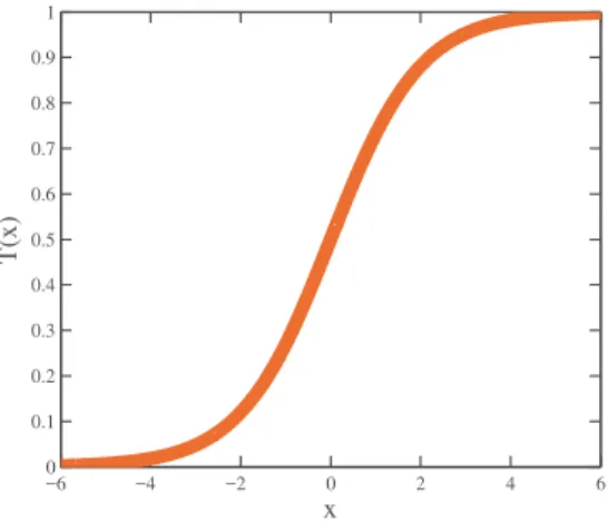
wherexdi(t+ 1)is the i−th element atdth dimension inx solution. This function is depicted
in Fig. 2. −6 −4 −2 0 2 4 6 0 0.1 0.2 0.3 0.4 0.5 0.6 0.7 0.8 0.9 1 x T(x)
Figure 2: Transfer Function.
4. The Proposed Approach
Population-based metaheuristics divide the search for the global optima into two phases, exploration (diversification) and exploitation (intensification). In exploration phase, the optimizer tries to explore the search space as much as possible in the hope to find more promising regions, while in the exploitation it tries to dig the neighborhood area of a specific solution in the hope of finding the global minimum. To avoid stagnation at the local mini-mum, the optimizer allows more exploration in the first stages of the optimization process, while in the later stages, more exploitation is allowed.
In the basic SSA, there is only one leader, who is responsible for exploiting the
neighbor-hood of the best solution (F), while the other N −1 individuals in the population
(follow-ers) are used to explore the search space. This mechanism might drive other salps toward locally optimal solutions when solving high-dimensional problems with a large number of local optima. This drawback motivated our attempt to divide the population into multiple sub-swarms with different leading salps to achieve more balance between exploration and
Accepted Manuscript
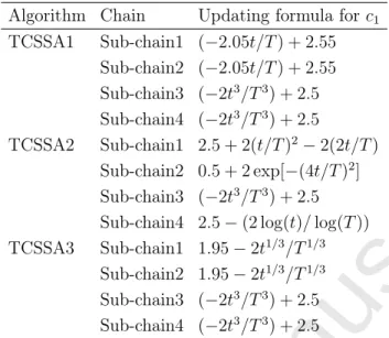
Table 1: Updating strategies
Algorithm Chain Updating formula forc1
TCSSA1 Sub-chain1 (−2.05t/T) + 2.55 Sub-chain2 (−2.05t/T) + 2.55 Sub-chain3 (−2t3/T3) + 2.5 Sub-chain4 (−2t3/T3) + 2.5 TCSSA2 Sub-chain1 2.5 + 2(t/T)2−2(2t/T) Sub-chain2 0.5 + 2 exp[−(4t/T)2] Sub-chain3 (−2t3/T3) + 2.5
Sub-chain4 2.5−(2 log(t)/log(T))
TCSSA3 Sub-chain1 1.95−2t1/3/T1/3
Sub-chain2 1.95−2t1/3/T1/3
Sub-chain3 (−2t3/T3) + 2.5
Sub-chain4 (−2t3/T3) + 2.5
exploitation. In this work, extensive experiments are conducted to set the best number of leaders that may lead to better performance than the basic SSA.
In the basic SSA, all salps behave the same and considered as one group, and one strategy is employed to update their positions. Theoretically, dividing the salps in SSA into many subgroups (sub-chains) with the same target (finding the best solution) could result in en-hancing the efficiency of the SSA in exploration and exploitation phases, simultaneously. In
this paper, different strategies are utilized for updating the c1 parameter to make a more
stable balance between the global and local search.
4.1. Updating strategies
In this paper, several strategies with different behaviors are utilized for updating the
c1 parameter in SSA. In each strategy, different functions with different properties (i.e.,
slopes, curvatures, and interception points) are employed to investigate their influence on
the performance of SSA. Those functions are reported in Table 1, where T represents the
max number of iterations and t shows the current iteration. These functions consist of
descending linear and polynomial, as well as exponential and logarithmic functions and their
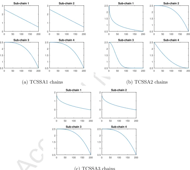
mathematical behaviors can be seen in Fig. 3. As may be observed in Fig. 3,c1 is decreased
over the iterations. It is clear that salps tend to have higher global search capability at the
beginning of the optimization when c1 values are close to the upper limit (2), while more
local search capability is allowed at the final stages. The basic idea of dividing the salp chain into four sub-chains is inspired from the behavior of termite colonies in exploring/exploiting the search space. Thus, three different versions of the SSA are proposed in this paper, which were named as TCSSA1, TCSSA2, and TCSSA3.
As it can be seen, in the TCSSA1 algorithm, two linear relations are utilized for group 1, in addition to linear and cubic rules for the next strategies, and 2 cubic rules for the third strategy. The TCSSA2 variant employs logarithmic, cubic, exponential, and quadratic rules for its strategies. These rules can generate different exploratory and exploitative temporal patterns that can be changed during the searching period. For example, salps that use rule
Accepted Manuscript
0 50 100 150 200 0 1 2 3 Sub-chain 1 0 50 100 150 200 0 1 2 3 Sub-chain 2 0 50 100 150 200 0.5 1 1.5 2 2.5 Sub-chain 3 0 50 100 150 200 0.5 1 1.5 2 2.5 Sub-chain 4(a) TCSSA1 chains
0 50 100 150 200 0.5 1 1.5 2 2.5 Sub-chain 1 0 50 100 150 200 0.5 1 1.5 2 2.5 Sub-chain 2 0 50 100 150 200 0.5 1 1.5 2 2.5 Sub-chain 3 0 50 100 150 200 0.5 1 1.5 2 2.5 Sub-chain 4 (b) TCSSA2 chains 0 50 100 150 200 -1 0 1 2 Sub-chain 1 0 50 100 150 200 -1 0 1 2 Sub-chain 2 0 50 100 150 200 0.5 1 1.5 2 2.5 Sub-chain 3 0 50 100 150 200 0.5 1 1.5 2 2.5 Sub-chain 4 (c) TCSSA3 chains
Accepted Manuscript
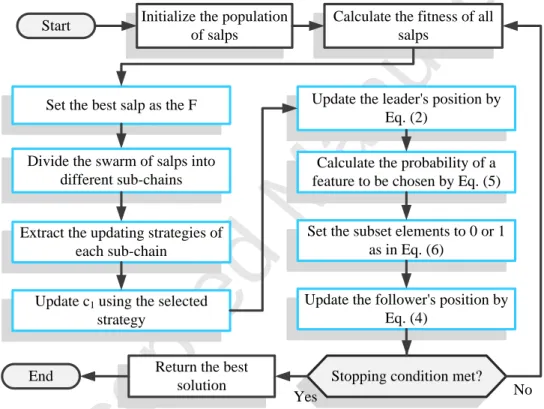
1 in the TCSSA2 version tend to switch the exploration and exploitation tendencies earlier than salps use rule 2. The TCSSA3 also utilizes a series of principal third root and cubic rules for updating its behaviors. In SSA with dynamic updating strategies (TCSSA) (see Fig. 4), first, a set of salps is randomly generated in the problem search space to initialize the population. After that, the particles are randomly divided into some predefined autonomous groups. At each iteration, the fitness value of each salp is calculated and the minimum value
is denoted as F. For each salp, the parameter c1 is updated using one of the four updating
strategies. After calculating the c1 value, the positions of salps will be updated using Eqs.
2 and 4. Then, the leader’s location (produced from 2) is converted to binary using Eqs. 5 and 6. Algorithm 2 shows the pseudo-code of the proposed TCSSA.
Initialize the population of salps
Set the best salp as the F
Calculate the probability of a feature to be chosen by Eq. (5)
Set the subset elements to 0 or 1 as in Eq. (6)
Update the follower's position by Eq. (4)
Stopping condition met? Start
Yes No
Calculate the fitness of all salps
Return the best solution End
Update c1 using the selected
strategy
Divide the swarm of salps into different sub-chains
Extract the updating strategies of each sub-chain
Update the leader's position by Eq. (2)
Figure 4: Flowchart of the proposed TCSSA algorithm
4.2. The proposed SSA for FS problems
The proposed wrapper-based FS technique utilizes the SSA-based algorithm as the
search-ing process and k-NN classifier as an evaluator. We first investigated the best number of
leaders, and we found that using half of the population (N/2) as leaders and the remaining
salps as followers leads to the best performance of the algorithm, thus BSSA usesN/2 salps
as leaders in all experiments. Then, three different updating strategies were used to
adap-tively update the c1 parameter in BSSA, namely TCSSA1, TCSSA2, TCSSA3. To design
the objective function of the FS task, two main points should be addressed initially: how to model the solutions and how to assess them.
In this paper, a feature subset is modeled as a binary vector. The length of this vector is equal to the number of features in the problem. When the feature is selected, the value is
Accepted Manuscript
Algorithm 2 Pseudo-code of the modified SSA algorithm
Initialize the salp population xi(i= 1,2, . . . , n)considering ub and lb
while (stopping condition is not met) do
Calculate the fitness of each salp
Set F as the best search agent
Divide the population of salps into different sub-chains
for (each salp (xi))do
if (i≤N/2) then
Extract the updating strategies of salps
Updatec1 using the selected strategy
Update the leader’s position by Eq. 2 Calculate the probability of a feature to be selected using Eq. 5
Set the subset elements to 0 or 1 as in Eq. 6
else
Update the follower’s position by Eq. 4
ReturnF
1; otherwise, it is assigned by 0. Two criteria are utilized to judge the excellence of a feature subset: the minimum inaccuracy rate (maximum classification accuracy) and the minimum number of selected features. These oppose objectives are assembled in the form of a fitness function. This function is demonstrated in Eq. 7:
↓F itness =αγR(D) +β
|R|
|C| (7)
whereγR(D)shows the classification error value of the classifier,|R|is the number of selected
features in a reduct, and |C| is the number of conditional features in the dataset, and
α∈[1,0], β= (1−α)are factors to show the prominence of quality and subset length based
on the observation and recommendations in [16].
5. Experimental Results and Discussion
This section summarizes the results of the proposed SSA with dynamic updating strate-gies for different feature selection datasets.
Data Sets: Table 3 shows the details of 20 well-regarded data sets that have been uti-lized in this work to evaluate the efficiencies of algorithms. This set of problems from UCI repository [40] covers a large variety of characteristics with different features and instances.
Experiment settings: An initial empirical study is presented to assess the influence of both
α and β on the performance of the proposed approach. Different values for α and β were
used to measure the fitness, accuracy, and reduction rates to locate the best combination. Colon dataset sample was used in all experiments. Table 2 shows the accuracy, fitness, and
reduction rates with different combinations of α and β values.
Inspecting the results in Table 2, it can be seen that accuracy rate and fitness, and
Accepted Manuscript
obtained when α = 0.99 and β = 0.01. The study’s summary is compatible with the values
that are commonly used in literature as well [67].
Table 2: Impact ofαandβ on the fitness, accuracy and Red. rate results based on Colon dataset.
α β Fitness Accuracy Red. rate
0.80 0.20 0.22583 0.83077 43.08961 0.60 0.40 0.29625 0.76154 45.76281 0.40 0.60 0.26798 0.80000 44.14000 0.20 0.80 0.28612 0.80000 44.26250 0.99 0.01 0.15633 0.84615 46.04657 0.96 0.04 0.16108 0.84615 44.77375 0.93 0.07 0.24922 0.76923 43.22441
For comparisons, we used three different optimizers: Binary Gravitational Search Algo-rithm (BGSA), Binary Bat AlgoAlgo-rithm (BBA), and binary Grey Wolf Optimizer (bGWO). The details of parameters of these optimizers are outlined in Table 4. The values have been selected based on both some initial simulations and previous researches. The proposed algo-rithms are evaluated to determine the superior reduct according to the error values of KNN
classifier having a Euclidean distance measure (K = 5 [16]). To study the optimality of
the solutions and validate the exploration and exploitation tendencies of optimizers, 80% of instances in every case were employed for training and the rest of them was used for testing stage [25].
System details: All results are computed in a same condition using MATLAB 2013 and a system with Intel Core(TM) i5-5200U 2.2GHz CPU and 4.0GB RAM.
Table 3: List of used datasets
No. Dataset No. of Features No. of instances
1. Exactly 13 1000 2. Exactly2 13 1000 3. HeartEW 13 270 4. Lymphography 18 148 5. M-of-n 13 1000 6. PenglungEW 325 73 7. SonarEW 60 208 8. SpectEW 22 267 9. CongressEW 16 435 10. IonosphereEW 34 351 11. KrvskpEW 36 3196 12. Tic-tac-toe 9 958 13. Vote 16 300 14. WaveformEW 40 5000 15. WineEW 13 178 16. Zoo 16 101 17. Clean1 166 476 18. Semeion 265 1593 19. Colon 2000 62 20. Leukemia 7129 72
Accepted Manuscript
Table 4: Parameter settings
Parameter Value
Population size 10
Number of iteration 100
Dimension Number of features
Number of runs for each technique 30
αin fitness function 0.99
β in fitness function 0.01
ain GWO [2 0]
QminFrequency minimum in BBA 0
QmaxFrequency maximum in BBA 2
ALoudness in BBA 0.5
r Pulse rate in BBA 0.5
G0in GSA 100
αin GSA 20
Results and discussion: Table 5 compares the average fitness results of BSSA with
differ-ent number of leaders fromN/2 toN/10. Based on the Friedman non-parametric statistical
test (F-test) results, we found that using N/2 salps as the leaders of other individuals
re-sults in obtaining more promising solutions for BSSA compared to other alternatives. The average accuracy and feature reduction rates of the BSSA with different number of leaders
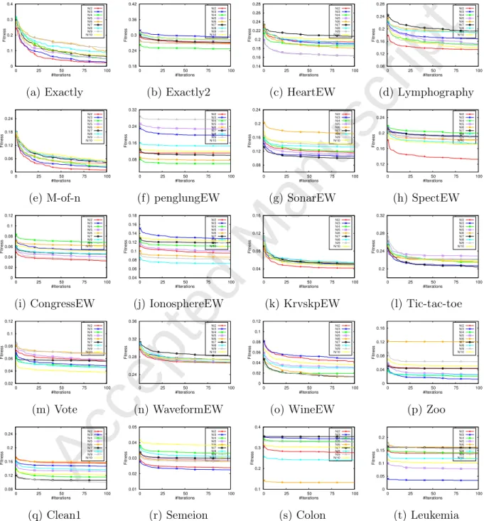
whenN=10 are demonstrated and compared graphically in Fig. 5. Figure 5 displays a color
representation (Heatmap) of the values of accuracy, reduction rate, and number of leaders, and F-test ranking over all datasets. Using these abstract graphical representations, several algorithms can be simultaneously judged in terms of different metrics.
As per accuracy results in Fig. 5a and in accordance with the reflected results in Table
5, for majority of datasets such as M-of-n, Exactly, and Semeion, the version with N/2
leaders has been colored by lighter degrees, which reveals the superiority of the BSSA with
N/2 salps compared to other versions. According to the ranking results (F-test) reported
in the top of Fig. 5a, the BSSA with N/2 salps has attained higher accuracies and as a
result, it has obtained the best place among other versions. The reason of these observations
is that the multi-leader structure with N/2 salps has effectively extended the exploitative
searching patterns of the BSSA; hence, it can show a successful performance in balancing the exploration and exploitation tendencies and jumping out of LO, whereas the other variants with different number of leaders still were susceptible to LO stagnation.
According to the reduction rates exposed in Fig. 5b, it is observed that they are scattered between 30% to 50% for the majority of datasets, and those values have been colored by
lighter degrees. The F-test ranking of the reduction rate results of the BSSA withN/6 salps,
N/3 salps, andN/2 salps are close to each other. It is detected that different variants reveal
a competitive efficacy and the distribution of colors cannot indicate a great gap between the rates of different alternatives. As a summary, the proposed approach considers both objec-tives (accuracy and feature reduction rate), to compromise between those two objecobjec-tives,
each objective has an impact level by settingα andβ coefficients. Since we are interested in
the accuracy objective (α=0.99) much higher than the reduction rates (β=0.01), we chose
the appropriate number of leaders (N/2) based on the F-test ranking of the accuracy results.
Accepted Manuscript
of leaders are demonstrated in Fig. 6. From Fig. 6, it can be observed that the convergence
behaviors of BSSA with N/2 salps are more accelerated than other variants for Exactly,
Lymphography, M-of-n, SpectEW, CongressEW, KrvskpEW, and WaveformEW, which is consistent with the results in Table 5. The dissimilarities of the acceleration values in the experimented curves also reveal the substantial impact the number of leading salps on the quality of the selected features.
In this regard, and according to the main metrics such as classification accuracy and
fitness results, the version with N/2 salps as the leaders of swarm is adopted as the basic
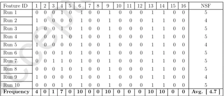
SSA approach (called BSSA), and considered as the base of the new improvements (using different updating strategies). Thus, the performance of BSSA is compared in terms of classification accuracy, fitness, and reduction rate (Red. Rate) to the binary algorithms with varied updating strategies in Table 6. From Table 6, it can be realized that the best optimizer in terms of accuracy and fitness measures is the TCSSA3. Based on the observed reduction rates, the best variants are the TCSSA1, TCSSA2, TCSSA3, and BSSA, respectively. Based on accuracy, the TCSSA3 can dominate other versions in dealing with 60% of datasets. It returns superior costs with acceptable STD values in the majority of cases. With regard to fitness values, it is superior to other techniques on the majority of problems. For Leukemia dataset, which has the highest number of features compared to other cases, the TCSSA3 algorithm has revealed the maximum accuracy 95.09 % and lowest fitness results indicating the advanced explorative and exploitative capacities of this version. According to the overall ranks, the TCSSA3 can be chosen as the peak method in terms of the main metrics. In addition, Table 7, Table 8, and Table 9 show a sample of the actual selected features with their frequency of ten runs for Exactly, SpectEW, and Zoo datasets.
The comparison of convergence rates is also provided in Fig. 7. From Fig. 7, it can be seen that for 55% of datasets, the TCSSA3 algorithm outperforms other versions in terms of fitness and accuracy, the convergence rate is also superior, and for the rest of cases, it has a competitive speed compared to the TCSSA1, which was also observed in Table 6. The results evidently show that the characteristics of the updating strategies can affect the exploratory and exploitative patterns SSA. The combination of exploratory and exploitative behaviors in the TCSSA3 can prevent salps from stagnation in locally optimal solutions. Hence, we can recognize a better efficacy of the TCSSA3 with the third group. Individual salps in the TCSSA3 can still strengthen the exploratory propensities even in the latter steps; enable it in avoiding the local optima (LO) and immature convergence drawbacks.
Table 10 compares the efficacy of TCSSA1 and TCSSA3 in terms of average and STD of measured metrics (i.e., fitness, accuracy and reduction rate) to those of other state-of-the-art techniques (i.e., bGWO, BGSA, and BBA). It is worth mentioning that those methods were implemented with the same parameter settings of BSSA based approaches (see Table 4), and used for comparison purposes. From Table 10, we can see that the performance of the proposed approaches in terms of average accuracy and fitness values are better than all other algorithms in 95% of datasets, where TCSSA1 obtained the best results in six datasets and TCSSA3 outperformed others in 14 datasets. Based on reduction rates, we observed that the BBA can slightly outperform other competitors.
Regarding the average accuracies, it can be observed that the TCSSA3 has reached to higher levels than 95% on Exactly, M-of-n, CongressEW, KrvskpEW, Vote, WineEW, Zoo, semeion, and Leukemia problems, while the second-best optimizer, bGWO, goes higher than
Accepted Manuscript
Table 5: The obtained results of the BSSA with different number of leaders based on average fitness results
Benchmark Metric N/2 N/3 N/4 N/5 N/6 N/7 N/8 N/9 N/10 Exactly AVG 0.02278 0.02605 0.04884 0.04999 0.09631 0.06280 0.08858 0.11940 0.06850 STD 0.02347 0.02262 0.04951 0.04625 0.07236 0.05025 0.06541 0.06821 0.04865 Exactly2 AVG 0.26964 0.29285 0.24746 0.28074 0.26787 0.27260 0.28357 0.26553 0.28382 STD 0.00656 0.01704 0.01723 0.00777 0.02501 0.01097 0.00984 0.01658 0.00453 HeartEW AVG 0.19466 0.19021 0.18614 0.16391 0.18094 0.20737 0.19184 0.16268 0.19888 STD 0.00726 0.01057 0.00482 0.00618 0.00826 0.01117 0.01393 0.00747 0.01305 Lymphography AVG 0.13389 0.16853 0.14983 0.15280 0.18755 0.19333 0.18821 0.14600 0.13912 STD 0.00830 0.01068 0.01371 0.01918 0.01654 0.02064 0.01672 0.02378 0.02176 M-of-n AVG 0.00899 0.02217 0.02558 0.04083 0.03812 0.04283 0.04581 0.04551 0.04857 STD 0.00830 0.01511 0.02208 0.02878 0.03396 0.03067 0.02859 0.03267 0.02848 penglungEW AVG 0.11125 0.19665 0.06036 0.22641 0.07693 0.10046 0.14550 0.27286 0.11881 STD 0.00523 0.00761 0.00490 0.01115 0.01219 0.01682 0.01108 0.01211 0.01467 SonarEW AVG 0.11559 0.10579 0.11965 0.11157 0.17110 0.10019 0.13206 0.13779 0.14074 STD 0.01041 0.01085 0.00975 0.01060 0.01285 0.01301 0.01340 0.01104 0.00742 SpectEW AVG 0.13271 0.19108 0.19959 0.18274 0.18294 0.19102 0.17342 0.18982 0.17172 STD 0.00884 0.00763 0.00823 0.01166 0.01024 0.00885 0.00953 0.01203 0.01502 CongressEW AVG 0.03243 0.05330 0.06819 0.04078 0.06177 0.04553 0.04607 0.03459 0.05146 STD 0.00473 0.00475 0.00601 0.00566 0.00612 0.00823 0.00589 0.00540 0.00847 IonosphereEW AVG 0.09549 0.12779 0.11092 0.10051 0.08622 0.11842 0.07252 0.08248 0.12242 STD 0.00775 0.01014 0.00741 0.00484 0.00627 0.00601 0.00655 0.00948 0.00813 KrvskpEW AVG 0.04130 0.05014 0.05228 0.05310 0.05286 0.05089 0.05409 0.04738 0.04608 STD 0.00526 0.00532 0.00700 0.00702 0.00698 0.00756 0.00711 0.00623 0.00664 Tic-tac-toe AVG 0.22161 0.20732 0.21500 0.22899 0.21483 0.20415 0.22065 0.22114 0.21756 STD 0.00000 0.00093 0.00477 0.00545 0.01159 0.00595 0.00501 0.00181 0.00665 Vote AVG 0.05735 0.04847 0.04629 0.05753 0.06864 0.05592 0.04595 0.06721 0.03806 STD 0.00605 0.00538 0.00574 0.00722 0.00668 0.00507 0.00454 0.00571 0.00675 WaveformEW AVG 0.26614 0.27395 0.26713 0.26860 0.27323 0.28225 0.27301 0.27331 0.27360 STD 0.00587 0.00510 0.00609 0.00504 0.00601 0.00554 0.00471 0.00503 0.00543 WineEW AVG 0.04276 0.04857 0.01923 0.03019 0.01294 0.01351 0.02981 0.01374 0.03633 STD 0.00387 0.00708 0.00039 0.00776 0.00693 0.00729 0.00083 0.00581 0.00811 Zoo AVG 0.04376 0.01257 0.02057 0.02593 0.12093 0.04339 0.02464 0.06376 0.05092 STD 0.00055 0.00909 0.00845 0.00092 0.00083 0.00072 0.00062 0.00070 0.00934 clean1 AVG 0.15544 0.14682 0.11538 0.13175 0.15706 0.10596 0.13619 0.10028 0.12149 STD 0.00572 0.00530 0.00616 0.00725 0.01131 0.00856 0.00624 0.00875 0.00803 semeion AVG 0.02385 0.02249 0.03313 0.02872 0.02804 0.02982 0.03108 0.02773 0.03807 STD 0.00109 0.00159 0.00172 0.00159 0.00152 0.00253 0.00178 0.00163 0.00196 Colon AVG 0.27648 0.34235 0.32776 0.41346 0.13261 0.35391 0.24054 0.32739 0.30188 STD 0.01807 0.01962 0.01765 0.01349 0.00095 0.00563 0.01518 0.00968 0.02062 Leukemia AVG 0.13811 0.03419 0.14084 0.07819 0.16191 0.15884 0.11704 0.15511 0.10072 STD 0.01007 0.00664 0.01581 0.01612 0.02303 0.01330 0.02025 0.01717 0.01331 W|T|L 7|0|13 3|0|17 2|0|18 0|0|20 2|0|18 2|0|18 1|0|19 2|0|18 1|0|19 F-Test 3.8 5.05 4.45 5.15 5.45 5.35 5.25 4.95 5.55
Accepted Manuscript
Exactly Exactly2 HeartEW Lymphography M-of-n PenglungEW SonarEW SpectEW CongressEW IonosphereEW KrvskpEW Tic-tac-toe Vote WaveformEW WineEW Zoo Clean1 Semeion Colon Leukemia N/2 N/3 N/4 N/5 N/6 N/7 N/8 N/9 N/10 Ranking(F-Test) 3.83 5.05 4.38 5.03 5.50 5.40 5.23 5.05 5.55 Datasets #No. of Leaders 0.7 0.75 0.8 0.85 0.9 0.95 1 Accuracy(a) Accuracy Results
1ing Exactly Exactly2 HeartEW Lymphography M-of-n penglungEW SonarEW SpectEW CongressEW IonosphereEW KrvskpEW Tic-tac-toe Vote WaveformEW WineEW Zoo clean1 semeion Colon Leukemia N/2 N/3 N/4 N/5 N/6 N/7 N/8 N/9 N/10 Ranking(F-Test) 4.75 4.70 5.10 5.85 3.60 4.45 6.10 4.80 5.65 Datasets #No. of Leaders 20 25 30 35 40 45 50 55 60 Reduction Rate (%)
Accepted Manuscript
0 0.1 0.2 0.3 0.4 0 25 50 75 100 Fitness #Iterations N/2 N/3 N/4 N/5 N/6 N/7 N/8 N/9 N/10 (a) Exactly 0.18 0.24 0.3 0.36 0.42 0 25 50 75 100 Fitness #Iterations N/2 N/3 N/4 N/5 N/6 N/7 N/8 N/9 N/10 (b) Exactly2 0.14 0.16 0.18 0.2 0.22 0.24 0.26 0.28 0 25 50 75 100 Fitness #Iterations N/2 N/3 N/4 N/5 N/6 N/7 N/8 N/9 N/10 (c) HeartEW 0.08 0.12 0.16 0.2 0.24 0.28 0 25 50 75 100 Fitness #Iterations N/2 N/3 N/4 N/5 N/6 N/7 N/8 N/9 N/10 (d) Lymphography 0 0.06 0.12 0.18 0.24 0 25 50 75 100 Fitness #Iterations N/2 N/3 N/4 N/5 N/6 N/7 N/8 N/9 N/10 (e) M-of-n 0.08 0.16 0.24 0.32 0 25 50 75 100 Fitness #Iterations N/2 N/3 N/4 N/5 N/6 N/7 N/8 N/9 N/10 (f) penglungEW 0.08 0.12 0.16 0.2 0.24 0 25 50 75 100 Fitness #Iterations N/2 N/3 N/4 N/5 N/6 N/7 N/8 N/9 N/10 (g) SonarEW 0.12 0.16 0.2 0.24 0 25 50 75 100 Fitness #Iterations N/2 N/3 N/4 N/5 N/6 N/7 N/8 N/9 N/10 (h) SpectEW 0 0.02 0.04 0.06 0.08 0.1 0.12 0 25 50 75 100 Fitness #Iterations N/2 N/3 N/4 N/5 N/6 N/7 N/8 N/9 N/10 (i) CongressEW 0.04 0.06 0.08 0.1 0.12 0.14 0.16 0.18 0 25 50 75 100 Fitness #Iterations N/2 N/3 N/4 N/5 N/6 N/7 N/8 N/9 N/10 (j) IonosphereEW 0.04 0.08 0.12 0.16 0 25 50 75 100 Fitness #Iterations N/2 N/3 N/4 N/5 N/6 N/7 N/8 N/9 N/10 (k) KrvskpEW 0.2 0.24 0.28 0.32 0 25 50 75 100 Fitness #Iterations N/2 N/3 N/4 N/5 N/6 N/7 N/8 N/9 N/10 (l) Tic-tac-toe 0.02 0.04 0.06 0.08 0.1 0.12 0 25 50 75 100 Fitness #Iterations N/2 N/3 N/4 N/5 N/6 N/7 N/8 N/9 N/10 (m) Vote 0.24 0.28 0.32 0.36 0 25 50 75 100 Fitness #Iterations N/2 N/3 N/4 N/5 N/6 N/7 N/8 N/9 N/10 (n) WaveformEW 0 0.02 0.04 0.06 0.08 0.1 0.12 0 25 50 75 100 Fitness #Iterations N/2 N/3 N/4 N/5 N/6 N/7 N/8 N/9 N/10 (o) WineEW 0 0.04 0.08 0.12 0.16 0 25 50 75 100 Fitness #Iterations N/2 N/3 N/4 N/5 N/6 N/7 N/8 N/9 N/10 (p) Zoo 0.08 0.12 0.16 0.2 0.24 0 25 50 75 100 Fitness #Iterations N/2 N/3 N/4 N/5 N/6 N/7 N/8 N/9 N/10 (q) Clean1 0.01 0.02 0.03 0.04 0.05 0 25 50 75 100 Fitness #Iterations N/2 N/3 N/4 N/5 N/6 N/7 N/8 N/9 N/10 (r) Semeion 0.1 0.2 0.3 0.4 0 25 50 75 100 Fitness #Iterations N/2 N/3 N/4 N/5 N/6 N/7 N/8 N/9 N/10 (s) Colon 0 0.05 0.1 0.15 0.2 0 25 50 75 100 Fitness #Iterations N/2 N/3 N/4 N/5 N/6 N/7 N/8 N/9 N/10 (t) LeukemiaAccepted Manuscript
0.95% only on three cases studies: semeion, Zoo, and WineEW datasets. However, in these cases, the classification rates of TCSSA3 are still higher than those of the bGWO. The average convergence speeds of different techniques can also be seen in Fig. 8. It can be detected that the TCSSA3 is capable of dominating other optimizers in the convergence accelerations on 18 datasets.
The main reason for the improved convergences and results is that the updating strategies in the TCSSA3 and the designed leadership structure can assist the binary algorithm in making a good balance between the exploratory and exploitative propensities. The faster convergence is due to the improved exploratory and exploitative capabilities of the TCSSA3 in exploiting the neighborhood of some leaders, while other leaders can travel to other fruitful regions of the feature space. As the results, SSA can discover better solutions quicker than other competitors. The notable improvements in the results have been achieved just by distributing the salp agents to a number of asynchronous cooperative teams by a variety of updating patterns instead of a single formulation for the main parameter in the SSA.
In Table 11, the average running time for the best TCSSA versions (i.e TCSSA1 and
TCSSA3), bGWO, BGSA, and BBA is reported for each dataset. It can be seen that
TCSSA3 is very competitive with the fastest algorithm which is BGSA. TCSSA3 has the second rank after BGSA over all datasets. This slight run time overhead in TCSSA variants is due to the incorporated mechanisms of updating rules and the new leadership structure.
Accepted Manuscript
T able 6: The results of the prop osed BSSA with differen t up dating approac hes Benc hmark Metric BSSA TCSSA1 TCSSA2 TCSSA3 Fitness A ccuracy Red. Rate Fitness A ccuracy Red. Rate Fitness A ccuracy Red. Rate Fitness A ccuracy Red. Rate Exactly A V G 0.02278 0.98253 43.88995 0.00881 0.99633 48.20513 0.00643 0.99873 48.20513 0.00811 0.99693 49.23077 STD 0.02347 0.02323 7.38679 0.00880 0.00860 4.48686 0.00567 0.00552 4.00639 0.00404 0.00381 3.83287 Exactly2 A V G 0.26964 0.73240 48.43495 0.24397 0.75973 38.97436 0.27167 0.73227 33.84615 0.23355 0.76720 69.23077 STD 0.00656 0.00620 12.21012 0.00311 0.00146 26.71831 0.00448 0.00435 5.92409 0.01406 0.01241 21.18698 HeartEW A V G 0.19466 0.80938 40.51164 0.17317 0.83111 40.25641 0.18855 0.81457 50.25641 0.17253 0.83309 27.17949 STD 0.00726 0.00699 6.88479 0.00530 0.00492 7.74078 0.01040 0.00962 12.24342 0.00715 0.00747 10.04648 Lymphograph y A V G 0.13389 0.87117 36.54285 0.13901 0.86486 47.77778 0.16338 0.84279 22.59259 0.16069 0.84437 33.88889 STD 0.00830 0.00850 7.89841 0.01339 0.01328 11.35742 0.00957 0.00971 4.36064 0.00812 0.00851 7.62996 M-of-n A V G 0.00899 0.99633 45.95979 0.00708 0.99827 46.41026 0.00590 0.99907 50.25641 0.00589 0.99920 48.97436 STD 0.00830 0.00812 4.44349 0.00370 0.00339 4.73037 0.00515 0.00511 3.90320 0.00332 0.00304 4.73037 p englungEW A V G 0.11125 0.89279 46.67115 0.08634 0.91892 39.27179 0.08650 0.91885 38.45128 0.09777 0.90721 40.93333 STD 0.00523 0.00493 5.25327 0.01380 0.01420 5.22264 0.00966 0.01005 5.85507 0.01643 0.01692 6.76753 SonarEW A V G 0.11559 0.89039 29.70496 0.07546 0.93045 34.00000 0.07235 0.93365 33.33333 0.05859 0.94808 28.16667 STD 0.01041 0.01059 6.66712 0.00812 0.00825 5.94676 0.01047 0.01052 6.94808 0.00577 0.00597 5.94273 Sp ectEW A V G 0.13271 0.87264 34.03079 0.17891 0.82537 39.69697 0.13190 0.87289 39.39394 0.17055 0.83333 44.54545 STD 0.00884 0.00875 7.01343 0.00760 0.00798 8.51911 0.01171 0.01151 11.53219 0.00712 0.00715 7.20185 CongressEW A V G 0.03243 0.97263 44.51875 0.04220 0.96223 51.87500 0.03246 0.97232 49.37500 0.03419 0.97049 50.20833 STD 0.00473 0.00458 8.02875 0.00421 0.00375 12.72957 0.00472 0.00458 8.26390 0.00473 0.00462 6.66375 IonosphereEW A V G 0.09549 0.91004 34.48902 0.12898 0.87519 45.78431 0.10324 0.90133 44.50980 0.06776 0.93769 39.31373 STD 0.00775 0.00805 8.28840 0.00936 0.00913 8.89703 0.00842 0.00850 7.97971 0.00542 0.00527 11.01797 KrvskpEW A V G 0.04130 0.96554 28.79408 0.04410 0.96197 35.46296 0.04147 0.96510 30.83333 0.03747 0.96923 29.90741 STD 0.00526 0.00523 4.17537 0.00563 0.00566 4.98419 0.00378 0.00381 6.41569 0.00470 0.00460 5.72925 Tic-tac-to e A V G 0.22161 0.78288 32.95411 0.20604 0.79749 44.44444 0.22257 0.78079 44.44444 0.20826 0.79749 22.22222 STD 0.00000 0.00000 2.02751 0.00000 0.00000 0.00000 0.00000 0.00000 0.00000 0.00000 0.00000 0.00000 V ote A V G 0.05735 0.94733 44.93523 0.05840 0.94667 43.95833 0.06007 0.94422 51.45833 0.05037 0.95489 42.91667 STD 0.00605 0.00590 9.91560 0.00661 0.00655 14.81598 0.00523 0.00567 12.78588 0.00435 0.00417 8.32615 W a v eformEW A V G 0.26614 0.73893 25.98109 0.26579 0.73852 30.75000 0.26619 0.73835 28.50000 0.26795 0.73643 29.83333 STD 0.00587 0.00547 6.96457 0.00498 0.00498 6.05827 0.00469 0.00462 6.45275 0.00407 0.00406 7.36761 WineEW A V G 0.04276 0.96442 25.88054 0.01547 0.98914 52.82051 0.01419 0.99138 43.33333 0.00810 0.99775 41.28205 STD 0.00387 0.00426 4.87576 0.00487 0.00465 8.26350 0.00842 0.00869 7.68789 0.00445 0.00457 6.54067 Zo o A V G 0.04376 0.96078 50.43375 0.07530 0.92941 45.83333 0.04965 0.95490 50.00000 0.01251 0.99281 46.04167 STD 0.00055 0.00000 5.65014 0.00892 0.00977 10.16212 0.00870 0.00914 7.34025 0.00905 0.00961 7.60759 clean1 A V G 0.15544 0.85014 30.31798 0.09826 0.90728 35.26104 0.12070 0.88515 30.02008 0.09267 0.91359 28.79518 STD 0.00572 0.00566 6.87348 0.00526 0.00551 5.72750 0.00500 0.00510 4.82728 0.00558 0.00581 5.34240 semeion A V G 0.02385 0.98344 27.28256 0.02146 0.98519 31.93711 0.02935 0.97737 30.50314 0.02726 0.97996 25.69811 STD 0.00109 0.00125 7.08537 0.00127 0.00141 4.62325 0.00157 0.00149 5.34592 0.00151 0.00149 5.15730 Colon A V G 0.27648 0.72689 37.07359 0.22822 0.77527 42.62167 0.19582 0.80753 47.32333 0.34495 0.65699 46.31833 STD 0.01807 0.01843 8.24942 0.00578 0.00589 4.29187 0.00569 0.00589 4.04031 0.01519 0.01581 6.69491 Leuk emia A V G 0.13811 0.86574 43.89360 0.09259 0.91204 44.90345 0.11796 0.88704 38.74036 0.05450 0.95092 40.81919 STD 0.01007 0.01053 6.57479 0.01016 0.01053 5.71851 0.01403 0.01447 7.49406 0.01140 0.01195 7.36320 W|T|L 2|0|18 3|0|17 2|0|18 4|0|16 1|1|18 9|1|10 3|0|17 3|0|17 4|1|15 11|0|10 11|1|8 3|0|17 F-T est 2.8500 2.8000 2.9500 2.5500 2.6250 1.9000 2.7000 2.7000 2.4000 1.9000 1.8750 2.7500Accepted Manuscript
Table 7: The actual features selected by the TCSSA3 algorithm for Exactly dataset (NSF: Number of selected features) Feature ID 1 2 3 4 5 6 7 8 9 10 11 12 13 NSF Run 1 1 0 1 0 1 0 1 0 1 0 1 0 0 6 Run 2 1 0 1 0 1 0 1 0 1 0 1 0 0 6 Run 3 1 0 1 0 1 0 1 0 1 0 1 0 0 6 Run 4 1 0 1 0 1 0 1 0 1 0 1 0 0 6 Run 5 1 0 1 0 1 0 1 0 1 0 1 0 0 6 Run 6 1 0 1 0 1 0 1 0 1 0 1 0 0 6 Run 7 1 0 1 0 1 0 1 0 1 0 1 0 0 6 Run 8 1 0 1 0 1 0 1 0 1 0 1 0 0 6 Run 9 1 0 1 0 1 0 1 0 1 0 1 0 0 6 Run 10 1 0 1 0 1 0 1 0 1 0 1 0 0 6 Frequency 10 0 10 0 10 0 10 0 10 0 10 0 0 Avg. [ 6 ]
Table 8: The actual features selected by the TCSSA3 algorithm for SpectEW dataset
Feature ID 1 2 3 4 5 6 7 8 9 10 11 12 13 14 15 16 17 18 19 20 21 22 NSF Run 1 0 0 0 0 0 0 1 0 0 1 1 0 1 0 0 0 0 1 0 1 1 0 6 Run 2 0 1 0 0 0 0 0 0 0 1 1 0 1 0 0 0 0 1 1 0 1 1 7 Run 3 0 1 0 0 0 1 0 0 0 1 0 0 1 0 0 0 0 0 0 0 1 1 4 Run 4 0 0 0 0 1 0 0 1 0 1 0 0 0 0 0 1 1 0 0 1 1 1 6 Run 5 0 1 0 1 0 0 1 0 1 1 1 0 1 0 0 0 0 1 0 0 1 0 5 Run 6 0 0 0 0 0 1 0 0 0 1 0 0 1 0 0 0 0 0 0 0 1 1 4 Run 7 0 0 0 0 0 0 0 1 0 1 0 0 0 0 0 0 1 0 0 1 1 1 5 Run 8 0 0 1 0 0 0 0 1 0 1 1 0 0 0 0 0 0 0 1 0 1 1 5 Run 9 0 0 0 0 1 0 0 1 0 1 1 0 0 0 0 1 1 1 1 1 1 1 9 Run 10 0 0 0 0 0 0 0 0 0 1 0 0 1 0 0 0 1 0 0 0 1 1 5 Frequency 0 3 1 1 2 2 2 4 1 10 5 0 6 0 0 2 4 4 3 4 10 8 Avg. [ 5.6 ]
Table 9: The actual features selected by the TCSSA3 algorithm for Zoo dataset
Feature ID 1 2 3 4 5 6 7 8 9 10 11 12 13 14 15 16 NSF Run 1 0 0 0 1 0 1 0 0 1 0 0 0 1 1 0 0 5 Run 2 1 0 0 0 0 1 0 0 1 0 0 0 1 1 0 0 4 Run 3 1 0 0 1 0 1 0 0 1 0 0 0 1 1 0 0 5 Run 4 0 0 0 1 0 1 0 0 1 0 0 0 1 1 0 0 5 Run 5 1 0 0 0 0 1 0 0 1 0 0 0 1 1 0 0 4 Run 6 0 0 0 1 0 1 0 0 1 0 0 0 1 1 0 0 5 Run 7 0 0 1 1 0 1 0 0 1 0 0 0 1 1 0 0 5 Run 8 0 0 0 1 0 1 0 0 1 0 0 0 1 1 0 0 5 Run 9 1 0 0 0 0 1 0 0 1 0 0 0 1 1 0 0 4 Run 10 0 0 0 1 0 1 0 0 1 0 0 0 1 1 0 0 5 Frequency 4 0 1 7 0 10 0 0 10 0 0 0 10 10 0 0 Avg. [ 4.7 ]
Accepted Manuscript
0 0.1 0.2 0.3 0.4 0 25 50 75 100 Fitness #Iterations BSSA TCSSA1 TCSSA2 TCSSA3 (a) Exactly 0.18 0.24 0.3 0.36 0.42 0 25 50 75 100 Fitness #Iterations BSSA TCSSA1 TCSSA2 TCSSA3 (b) Exactly2 0.14 0.16 0.18 0.2 0.22 0.24 0.26 0.28 0 25 50 75 100 Fitness #Iterations BSSA TCSSA1 TCSSA2 TCSSA3 (c) HeartEW 0.08 0.12 0.16 0.2 0.24 0.28 0 25 50 75 100 Fitness #Iterations BSSA TCSSA1 TCSSA2 TCSSA3 (d) Lymphography 0 0.06 0.12 0.18 0.24 0 25 50 75 100 Fitness #Iterations BSSA TCSSA1 TCSSA2 TCSSA3 (e) M-of-n 0.08 0.16 0.24 0.32 0 25 50 75 100 Fitness #Iterations BSSA TCSSA1 TCSSA2 TCSSA3 (f) penglungEW 0 0.06 0.12 0.18 0.24 0 25 50 75 100 Fitness #Iterations BSSA TCSSA1 TCSSA2 TCSSA3 (g) SonarEW 0.12 0.16 0.2 0.24 0 25 50 75 100 Fitness #Iterations BSSA TCSSA1 TCSSA2 TCSSA3 (h) SpectEW 0 0.02 0.04 0.06 0.08 0.1 0.12 0 25 50 75 100 Fitness #Iterations BSSA TCSSA1 TCSSA2 TCSSA3 (i) CongressEW 0.04 0.06 0.08 0.1 0.12 0.14 0.16 0.18 0 25 50 75 100 Fitness #Iterations BSSA TCSSA1 TCSSA2 TCSSA3 (j) IonosphereEW 0.04 0.08 0.12 0.16 0 25 50 75 100 Fitness #Iterations BSSA TCSSA1 TCSSA2 TCSSA3 (k) KrvskpEW 0.2 0.24 0.28 0.32 0 25 50 75 100 Fitness #Iterations BSSA TCSSA1 TCSSA2 TCSSA3 (l) Tic-tac-toe 0.02 0.04 0.06 0.08 0.1 0.12 0 25 50 75 100 Fitness #Iterations BSSA TCSSA1 TCSSA2 TCSSA3 (m) Vote 0.24 0.28 0.32 0.36 0 25 50 75 100 Fitness #Iterations BSSA TCSSA1 TCSSA2 TCSSA3 (n) WaveformEW 0 0.02 0.04 0.06 0.08 0.1 0.12 0 25 50 75 100 Fitness #Iterations BSSA TCSSA1 TCSSA2 TCSSA3 (o) WineEW 0 0.04 0.08 0.12 0.16 0 25 50 75 100 Fitness #Iterations BSSA TCSSA1 TCSSA2 TCSSA3 (p) Zoo 0.08 0.12 0.16 0.2 0.24 0 25 50 75 100 Fitness #Iterations BSSA TCSSA1 TCSSA2 TCSSA3 (q) Clean1 0.01 0.02 0.03 0.04 0.05 0 25 50 75 100 Fitness #Iterations BSSA TCSSA1 TCSSA2 TCSSA3 (r) Semeion 0.1 0.2 0.3 0.4 0 25 50 75 100 Fitness #Iterations BSSA TCSSA1 TCSSA2 TCSSA3 (s) Colon 0 0.05 0.1 0.15 0.2 0 25 50 75 100 Fitness #Iterations BSSA TCSSA1 TCSSA2 TCSSA3 (t) LeukemiaFigure 7: Convergence curves for BSSA withN/2 leaders and proposed updating approaches for all
Accepted Manuscript
0 0.1 0.2 0.3 0.4 0 25 50 75 100 Fitness #Iterations TCSSA3 bGWO BGSA BBA (a) Exactly 0.18 0.24 0.3 0.36 0.42 0 25 50 75 100 Fitness #Iterations TCSSA3 bGWO BGSA BBA (b) Exactly2 0.14 0.16 0.18 0.2 0.22 0.24 0.26 0.28 0 25 50 75 100 Fitness #Iterations TCSSA3 bGWO BGSA BBA (c) HeartEW 0.08 0.12 0.16 0.2 0.24 0.28 0 25 50 75 100 Fitness #Iterations TCSSA3 bGWO BGSA BBA (d) Lymphography 0 0.06 0.12 0.18 0.24 0 25 50 75 100 Fitness #Iterations TCSSA3 bGWO BGSA BBA (e) M-of-n 0.08 0.16 0.24 0.32 0 25 50 75 100 Fitness #Iterations TCSSA3 bGWO BGSA BBA (f) penglungEW 0 0.06 0.12 0.18 0.24 0 25 50 75 100 Fitness #Iterations TCSSA3 bGWO BGSA BBA (g) SonarEW 0.12 0.16 0.2 0.24 0 25 50 75 100 Fitness #Iterations TCSSA3 bGWO BGSA BBA (h) SpectEW 0 0.02 0.04 0.06 0.08 0.1 0.12 0 25 50 75 100 Fitness #Iterations TCSSA3 bGWO BGSA BBA (i) CongressEW 0.04 0.06 0.08 0.1 0.12 0.14 0.16 0.18 0 25 50 75 100 Fitness #Iterations TCSSA3 bGWO BGSA BBA (j) IonosphereEW 0.04 0.08 0.12 0.16 0 25 50 75 100 Fitness #Iterations TCSSA3 bGWO BGSA BBA (k) KrvskpEW 0.2 0.24 0.28 0.32 0 25 50 75 100 Fitness #Iterations TCSSA3 bGWO BGSA BBA (l) Tic-tac-toe 0.02 0.04 0.06 0.08 0.1 0.12 0 25 50 75 100 Fitness #Iterations TCSSA3 bGWO BGSA BBA (m) Vote 0.24 0.28 0.32 0.36 0 25 50 75 100 Fitness #Iterations TCSSA3 bGWO BGSA BBA (n) WaveformEW 0 0.02 0.04 0.06 0.08 0.1 0.12 0 25 50 75 100 Fitness #Iterations TCSSA3 bGWO BGSA BBA (o) WineEW 0 0.04 0.08 0.12 0.16 0 25 50 75 100 Fitness #Iterations TCSSA3 bGWO BGSA BBA (p) Zoo 0.08 0.12 0.16 0.2 0.24 0 25 50 75 100 Fitness #Iterations TCSSA3 bGWO BGSA BBA (q) Clean1 0.01 0.02 0.03 0.04 0.05 0 25 50 75 100 Fitness #Iterations TCSSA3 bGWO BGSA BBA (r) Semeion 0.1 0.2 0.3 0.4 0 25 50 75 100 Fitness #Iterations TCSSA3 bGWO BGSA BBA (s) Colon 0 0.05 0.1 0.15 0.2 0 25 50 75 100 Fitness #Iterations TCSSA3 bGWO BGSA BBA (t) LeukemiaAccepted Manuscript
T able 10: Comparison b et w e en the TCSSA 1 , TCSSA3 and other metaheuristics a p pro ac hes based on the a v erage fitness, a v erage accuracy , and a v erage features reduction rate results. Benc hmark Metric TCSSA1 TCSSA3 bGW O BGSA BBA Fitness A ccuracy Red. Rate Fitness A ccuracy Red. Rate Fitness A ccuracy Red. Rate Fitness A ccuracy Red. Rate Fitness A ccuracy Red. Rate Exactly A V G 0.00881 0.9963 3 48.20513 0.00811 0.99693 49.23077 0.19650 0.80947 21.2820 5 0.30655 0.69713 32.82051 0.32331 0.60993 55.89744 STD 0.00880 0.0086 0 4.48686 0.00404 0.00381 3.83287 0.07663 0.07622 12.7255 5 0.05933 0.06012 8.06354 0.07446 0.06467 14.5578 0 Exactly2 A V G 0.24397 0.7597 3 38.97436 0.23355 0.76720 69.23077 0.25994 0.74313 43.5897 4 0.29485 0.70613 60.76923 0.32592 0.62820 53.3333 3 STD 0.00311 0.0014 6 26.71831 0.01406 0.01241 21.18698 0.01924 0.01723 31.9618 6 0.02409 0.02348 16.20492 0.01671 0.05735 17.9474 5 HeartEW A V G 0.17317 0.8311 1 40.25641 0.17253 0.83309 27.17949 0.21259 0.79161 37.1794 9 0.22599 0.77704 47.43590 0.20840 0.75383 54.61538 STD 0.00530 0.0049 2 7.74078 0.00715 0.00747 10.04648 0.01701 0.01693 15.3956 6 0.02139 0.02160 10.11731 0.01468 0.03259 12.6720 0 Lymphograph y A V G 0.13901 0.86486 47.77778 0.16069 0.84437 33.88889 0.19124 0.81306 38.3333 3 0.22182 0.78108 49.07407 0.22615 0.70135 56.66667 STD 0.01339 0.0132 8 11.35742 0.00812 0.00851 7.62996 0.02813 0.02841 10.9519 2 0.02151 0.02170 10.52914 0.02365 0.06903 12.2413 6 M-of-n A V G 0.00708 0.9982 7 46.41026 0.00589 0.99920 48.97436 0.11222 0.89413 25.8974 4 0.16966 0.83520 34.87179 0.17141 0.72187 52.56410 STD 0.00370 0.0033 9 4.73037 0.00332 0.00304 4.73037 0.04149 0.04120 7.41773 0.06254 0.06320 11.01525 0.05619 0.07971 16.0446 4 p englungEW A V G 0.08634 0.91892 39.27179 0.09777 0.90721 40.9333 3 0.15406 0.84955 48.8205 1 0.08511 0.91892 51.64103 0.16835 0.79459 61.17949 STD 0.01380 0.0142 0 5.22264 0.01643 0.01692 6.76753 0.01300 0.01362 8.68683 0.00024 0.00000 2.37800 0.01690 0.02892 4.80025 SonarEW A V G 0.07546 0.9304 5 34.00000 0.05859 0.94808 28.16667 0.16882 0.83558 39.6111 1 0.11638 0.88750 49.94444 0.11012 0.84391 58.83333 STD 0.00812 0.0082 5 5.94676 0.00577 0.00597 5.94273 0.01594 0.01604 14.3551 2 0.01483 0.01497 6.16633 0.02095 0.03595 8.96086 Sp ectEW A V G 0.17891 0.8253 7 39.69697 0.17055 0.83333 44.54545 0.19414 0.80970 42.5757 6 0.21957 0.78259 56.66667 0.17164 0.79975 63.78788 STD 0.00760 0.0079 8 8.51911 0.00712 0.00715 7.20185 0.01362 0.01354 11.1009 3 0.02411 0.02414 10.45648 0.01191 0.02652 10.3709 6 CongressEW A V G 0.04220 0.9622 3 51.87500 0.03419 0.97049 50.20833 0.05648 0.94755 54.3750 0 0.05252 0.95122 57.70833 0.06443 0.87171 61.04167 STD 0.00421 0.0037 5 12.72957 0.00473 0.00462 6.66375 0.01094 0.01069 13.3493 8 0.00832 0.00812 15.01466 0.01470 0.07533 12.8908 0 IonosphereEW A V G 0.12898 0.8751 9 45.78431 0.06776 0.93769 39.31373 0.11984 0.88466 43.4313 7 0.12209 0.88125 54.70588 0.10764 0.87652 60.58824 STD 0.00936 0.0091 3 8.89703 0.00542 0.00527 11.01797 0.00890 0.00934 14.7501 0 0.01037 0.01048 7.39239 0.01184 0.01899 7.63066 KrvskpEW A V G 0.04410 0.9619 7 35.46296 0.03747 0.96923 29.90741 0.07304 0.93390 23.9814 8 0.09655 0.90807 44.53704 0.11737 0.81635 58.33333 STD 0.00563 0.0056 6 4.98419 0.00470 0.00460 5.72925 0.01500 0.01457 9.41237 0.04729 0.04784 5.90308 0.04677 0.08068 7.92418 Tic-tac-to e A V G 0.20604 0.79749 44.44444 0.20826 0.79749 22.22222 0.25119 0.75379 25.5555 6 0.25144 0.75261 34.81481 0.25680 0.66535 47.77778 STD 0.00000 0.0000 0 0.00000 0.00000 0.00000 0.00000 0.03221 0.03224 14.9213 9 0.02366 0.02442 12.62935 0.02374 0.06277 16.5448 9 V ote A V G 0.05840 0.9466 7 43.95833 0.05037 0.95489 42.91667 0.06029 0.94378 53.7500 0 0.07308 0.93133 48.95833 0.07122 0.85111 61.66667 STD 0.00661 0.0065 5 14.81598 0.00435 0.00417 8.32615 0.01033 0.00985 13.8884 1 0.01093 0.01109 11.38134 0.01298 0.09571 13.6075 4 W a v eformEW A V G 0.26579 0.73852 30.75000 0.26795 0.73643 29.83333 0.28250 0.72272 20.0833 3 0.30732 0.69460 50.25000 0.30371 0.66931 58.33333 STD 0.00498 0.0049 8 6.05827 0.00407 0.00406 7.36761 0.00725 0.00674 11.5311 3 0.01399 0.01422 7.29165 0.01354 0.03258 8.26118 WineEW A V G 0.01547 0.9891 4 52.82051 0.00810 0.99775 41.28205 0.04666 0.95955 33.8461 5 0.05424 0.95094 43.33333 0.03647 0.91873 53.33333 STD 0.00487 0.0046 5 8.26350 0.00445 0.00457 6.54067 0.01167 0.01165 13.4908 7 0.01514 0.01547 8.44666 0.01300 0.05193 13.3896 7 Zo o A V G 0.07530 0.9294 1 45.83333 0.01251 0.99281 46.04167 0.03171 0.97451 35.2083 3 0.06528 0.93922 48.95833 0.04153 0.87386 58.95833 STD 0.00892 0.0097 7 10.16212 0.00905 0.00961 7.60759 0.00850 0.00914 15.5262 7 0.00782 0.00789 7.35553 0.01487 0.09490 15.6300 3 clean1 A V G 0.09826 0.9072 8 35.26104 0.09267 0.91359 28.79518 0.09868 0.90770 26.9477 9 0.10584 0.89818 49.57831 0.15587 0.82647 60.98394 STD 0.00526 0.0055 1 5.72750 0.00558 0.00581 5.34240 0.00621 0.00619 12.4646 9 0.01044 0.01056 3.26580 0.01297 0.02082 6.03382 semeion A V G 0.02146 0.98519 31.93711 0.02726 0.97996 25.69811 0.03562 0.97164 24.4905 7 0.03365 0.97110 49.61006 0.03343 0.96219 59.61006 STD 0.00127 0.0014 1 4.62325 0.00151 0.00149 5.15730 0.00259 0.00298 11.7064 4 0.00201 0.00215 2.80073 0.00262 0.00629 4.13076 Colon A V G 0.22822 0.77527 42.62167 0.34495 0.65699 46.31833 0.34053 0.66129 47.8950 0 0.23704 0.76559 50.20833 0.27856 0.68172 58.62500 STD 0.00578 0.0058 9 4.29187 0.01519 0.01581 6.69491 0.02175 0.02201 6.33605 0.01435 0.01451 1.00104 0.03524 0.03763 2.76853 Leuk emia A V G 0.09259 0.9120 4 44.90345 0.05450 0.95092 40.81919 0.11972 0.88426 48.6075 7 0.15990 0.84352 50.13139 0.08452 0.87685 59.88217 STD 0.01016 0.0105 3 5.71851 0.01140 0.01195 7.36320 0.01617 0.01645 4.13624 0.01345 0.01362 0.55706 0.02291 0.02889 3.47373 W|T|L 5|0|13 4|2|14 0|0|20 0|0|20 14|1|5 1|0|19 0|0|20 0|0|20 0|0|20 1|0|19 0|1|19 0|0|20 0|0|20 0|0|20 19|0|1 F-T est 2.150 2.050 3.55000 3.500 1.475 3.95000 3.500 3.100 4.05000 4.000 3.675 2.35000 3.850 4.700 1.10000Accepted Manuscript
Table 11: Comparison between the TCSSA1, TCSSA3 and other metaheuristics approaches based on the average running time results.
Benchmark TCSSA1 TCSSA3 bGWO BGSA BBA
AVG STD AVG STD AVG STD AVG STD AVG STD
Exactly 5.5835 0.2267 6.0734 0.3506 6.1544 0.2753 4.8760 0.3113 4.9563 0.2719 Exactly2 5.8795 0.4261 5.5584 0.4304 6.0499 0.3798 5.0329 0.3743 5.2239 0.3941 HeartEW 2.8059 0.1323 2.6691 0.1525 2.7390 0.1737 2.8118 0.1822 2.7666 0.2005 Lymphography 2.5142 0.1165 2.3768 0.1149 2.6023 0.1607 2.5885 0.1496 2.6343 0.1452 M-of-n 5.5922 0.2521 5.5850 0.2444 6.1569 0.2410 5.1377 0.2934 4.8916 0.3614 penglungEW 4.0432 0.1659 4.0211 0.2190 7.7166 0.4321 3.0602 0.1707 4.1657 0.2384 SonarEW 2.9612 0.1461 2.8761 0.1465 3.6772 0.1928 2.7028 0.1462 2.8501 0.1910 SpectEW 2.6541 0.1526 2.7215 0.1789 2.8694 0.1757 2.7225 0.1621 2.8089 0.1613 CongressEW 3.2748 0.1734 3.3135 0.2262 3.3091 0.1719 3.2168 0.1878 3.2435 0.1582 IonosphereEW 3.1135 0.1653 3.2154 0.2275 3.5639 0.1838 2.9213 0.1445 3.0184 0.1479 KrvskpEW 62.5567 2.6913 66.8095 2.2950 78.1132 4.6058 49.5337 2.5273 47.9225 2.5762 Tic-tac-toe 4.9093 0.2508 5.2740 0.2704 6.2078 0.6220 4.3440 0.2784 4.2372 0.2775 Vote 2.8021 0.1291 2.6335 0.1352 2.8512 0.1536 2.8243 0.1516 2.8343 0.1783 WaveformEW 166.6715 4.8928 175.5412 6.1130 213.9553 13.6071 125.8036 6.7701 119.9900 8.1688 WineEW 2.5566 0.1297 2.4475 0.1276 2.6282 0.1734 2.5852 0.1706 2.6238 0.1408 Zoo 2.5131 0.1158 2.3792 0.1176 2.6234 0.1358 2.5473 0.1579 2.7774 0.1923 clean1 9.7487 0.2374 10.1214 0.3580 13.6825 0.6475 7.3968 0.2884 7.5886 0.4673 semeion 126.3091 1.9589 135.8338 2.6086 169.5376 9.1906 90.6010 2.2118 82.7761 5.5785 Colon 11.9469 0.4566 11.7073 0.5344 36.6944 1.9980 5.1536 0.2417 12.1760 0.7744 Leukemia 41.8940 1.8276 41.2598 1.7718 130.8780 6.3655 16.4414 0.6832 39.3789 2.4179 W|T|L 1|0|19 5|0|15 0|0|20 9|0|11 5|0|15 F-Test 2.950 2.800 4.700 1.950 2.600
Comparison with other meta-heuristics in literature: After analyzing the results of the proposed approaches, a comparison with similar approaches from the literature is given based on classification accuracy rates. The results for those approaches were obtained from two well-known research works that used the same datasets. In Table 12, we compared the performance of TCSSA3 with the results of GA and PSO from [37] executed using the source code from the same authors, the results of the bGWO1, bGWO2, GA, and PSO obtained from the paper [16], and a similar approach that uses the same updating strategy for the PSO algorithm (i.e., AGPSO3) proposed in [55].
Table 12 shows that TCSSA3 provides a superior performance in comparison with other approaches. It obtained the best results in 70% of the datasets with a significant difference according to the F-Test. Compared to the PSO1 and PSO2 approaches, TCSSA3 can out-perform both approaches in all datasets. The AGPSO3, which is an enhanced PSO approach that uses a similar updating strategy used in TCSSA3, comes in the second place after TC-SSA3. It can be seen that AGPSO3 performs better than both PSO approaches on fourteen datasets, which means that using different updating strategies with the PSO can enhance the performance of this algorithm on feature selection tasks. At the same time, AGPSO3 can outperform TCSSA3 in only four datasets. The previous results clearly prove the influence of different updating strategies on the capabilities of SSA in searching for the most informative features. The proposed SSA-based method can reveal the highest classification accuracies for different datasets with different dimensions.
The proposed asynchronous team behaviors of agents allow them to have a variety of ran-domized patterns in performing the socio-random exploration and exploitation phases for all search agents. This results in enhancements in local solutions avoidance of the TCSSA3 algorithm. We think that the proposed updating mechanisms and considering multi-leader structure can also expand the exploratory and exploitative capacities of the other stochas-tic optimizers. Interpretation of these effects for other population-based optimizers would
Accepted Manuscript
Table 12: Comparison between the TCSSA3 and other meta-heuristics from the literature in terms of accuracy
Benchmark TCSSA3 GA1 [37] PSO1 [37] bGWO1 [15] bGWO2 [15] GA2 [15] PSO2 [15] AGPSO3 [53]
Exactly 0.99693 0.82200 0.97327 0.70800 0.77600 0.67400 0.68800 1.00000 Exactly2 0.76720 0.67720 0.66640 0.74500 0.75000 0.74600 0.73000 0.76083 HeartEW 0.83309 0.73235 0.74469 0.77600 0.77600 0.78000 0.78700 0.79259 Lymphography 0.84437 0.75766 0.75946 0.74400 0.70000 0.69600 0.74400 0.82508 M-of-n 0.99920 0.91600 0.99620 0.90800 0.96300 0.86100 0.92100 1.00000 penglungEW 0.90721 0.67207 0.87928 0.60000 0.58400 0.58400 0.58400 0.83556 SonarEW 0.94808 0.83333 0.80353 0.73100 0.72900 0.75400 0.73700 0.88571 SpectEW 0.83333 0.75597 0.73806 0.82000 0.82200 0.79300 0.82200 0.70308 CongressEW 0.97049 0.89771 0.93746 0.93500 0.93800 0.93200 0.92800 0.96130 IonosphereEW 0.93769 0.86269 0.87614 0.80700 0.83400 0.81400 0.81900 0.89202 KrvskpEW 0.96923 0.94026 0.94875 0.94400 0.95600 0.92000 0.94100 0.96422 Tic-tac-toe 0.79749 0.76388 0.75024 0.72800 0.72700 0.71900 0.73500 0.81250 Vote 0.95489 0.80844 0.88844 0.91200 0.92000 0.90400 0.90400 0.96556 WaveformEW 0.73643 0.71207 0.73168 0.78600 0.78900 0.77300 0.76200 0.73827 WineEW 0.99775 0.94719 0.93670 0.93000 0.92000 0.93700 0.93300 0.96852 Zoo 0.99281 0.94575 0.96275 0.87900 0.87900 0.85500 0.86100 0.97059 W|T|L 11|0|5 0|0|16 0|0|16 0|0|16 1|0|15 0|0|16 0|0|16 4|0|12 F-Test 1.563 5.438 4.625 5.469 4.844 6.156 5.531 2.375
need deeper insight into the exploration and exploitation mechanisms of those algorithms supported by some experiments and analyses and will go far outside the core scope of this research.
6. Conclusion and future directions
In this work, an asynchronous binary SSA algorithm with several updating rules was proposed to tackle the FS problems. First, tests were performed to determine the best leadership structure of the artificial salp chains. SSA with the best leadership structure
(N/2 salps as leaders) was then used as the basic algorithm (BSSA) to implement the
following approaches. The whole chain was divided to several sub-chains, where the salps in each sub-chain could follow a different strategy to adaptively update their locations inside the search space. Three different updating strategies (TCSSA1, TCSSA2, TCSSA3) were used. In each strategy, each subchain of the salps followed an updating mechanism. The proposed algorithm was benchmarked on 20 datasets from UCI repository. The statistical results confirm the superiority of the proposed TCSSA3 in dealing with exploration and exploitation of the feature space for the majority of datasets. The discussions and analyses of results showed that idea of asynchronous tuning of the main parameter of the SSA with different leading salp for different regions of the salp chain is beneficial in alleviating the possible drawbacks of the conventional algorithm.
Future researches can investigate the optimum number of updating rules and utilize the proposed structure for other population-based algorithms.
7. Acknowledgements