Using Quantile Regression for Duration Analysis

econ

stor

www.econstor.eu

Der Open-Access-Publikationsserver der ZBW – Leibniz-Informationszentrum Wirtschaft The Open Access Publication Server of the ZBW – Leibniz Information Centre for Economics

Nutzungsbedingungen:

Die ZBW räumt Ihnen als Nutzerin/Nutzer das unentgeltliche, räumlich unbeschränkte und zeitlich auf die Dauer des Schutzrechts beschränkte einfache Recht ein, das ausgewählte Werk im Rahmen der unter

→ http://www.econstor.eu/dspace/Nutzungsbedingungen nachzulesenden vollständigen Nutzungsbedingungen zu vervielfältigen, mit denen die Nutzerin/der Nutzer sich durch die erste Nutzung einverstanden erklärt.

Terms of use:

The ZBW grants you, the user, the non-exclusive right to use the selected work free of charge, territorially unrestricted and within the time limit of the term of the property rights according to the terms specified at

→ http://www.econstor.eu/dspace/Nutzungsbedingungen By the first use of the selected work the user agrees and declares to comply with these terms of use.

Fitzenberger, Bernd; Wilke, Ralf A.

Working Paper

Using Quantile Regression for Duration

Analysis

ZEW Discussion Papers, No. 05-65

Provided in cooperation with:

Zentrum für Europäische Wirtschaftsforschung (ZEW)

Suggested citation: Fitzenberger, Bernd; Wilke, Ralf A. (2005) : Using Quantile Regression for Duration Analysis, ZEW Discussion Papers, No. 05-65, http://hdl.handle.net/10419/24161

Discussion Paper No. 05-65

Using Quantile Regression

for Duration Analysis

Discussion Paper No. 05-65

Using Quantile Regression

for Duration Analysis

Bernd Fitzenberger and Ralf A. Wilke

Die Discussion Papers dienen einer möglichst schnellen Verbreitung von neueren Forschungsarbeiten des ZEW. Die Beiträge liegen in alleiniger Verantwortung

der Autoren und stellen nicht notwendigerweise die Meinung des ZEW dar. Discussion Papers are intended to make results of ZEW research promptly available to other

Download this ZEW Discussion Paper from our ftp server:

Non–technical Summary

This survey summarizes recent estimation approaches using quantile regression for (right-censored) duration data. We provide a discussion of the advantages and drawbacks of quantile regression in comparison to popular alternative methods such as the (mixed-)proportional hazard model or the accelerated failure time model. We argue that quantile regression methods are robust and flexible in a sense that they can capture a variety of effects at different quantiles of the duration distribution. This survey discusses a selection of well known theoretical results and adds some new theoretical insights on the relationship between the proportional hazard rate model, the presence of unobserved heterogeneity, and the estimation of quantile regression. Our discussion emphasizes cases when evidence based on quantile regression implies a rejection of the proportional hazard model. Quantile regression also allow to estimate hazard rates which are often of interest in duration analysis and the method can be extended to a nonlinear Box-Cox transformation of the duration variable. Furthermore, the survey points out that quantile regression can not take account of time–varying covariates and it has not been extended so far to account for unobserved heterogeneity and competing risks.

We illustrate our theoretical reasoning by an application of the quantile regression to unem-ployment duration data for young workers in West-Germany. We find that some variables change the direction of their influence on unemployment duration across the distribution. This implies that the basic assumptions for a proportional hazard model is violated in our application. These empirical findings motivate the use of the estimation approaches discussed in this survey. Our results indicate that the overall unemployment rate shows no impact on the distribution of unem-ployment durations and that the duration of unemunem-ployment for young workers has become shorter over time.

Using Quantile Regression for Duration Analysis

∗

Bernd Fitzenberger

_{and Ralf A. Wilke}

August 2005

∗_{This is a longer version of our paper published (in: Allgemeines Statistisches Archiv 90(1)). Here, we add}

the discussion of Box-Cox quantile regression and the details of the empirical application. The paper benefitted from the helpful comments by an anonymous referee. We gratefully acknowledge financial support by the German Research Foundation (DFG) through the research project “Microeconometric modelling of unemployment durations under consideration of the macroeconomic situation”. Thanks are due to Eva M¨uller and Xuan Zhang for excellent research assistance. The empirical work in this paper uses partly the IAB employment subsample 19752001 -regional file - which is a 2% random sample of all employees in Germany who have been covered by the social insurance system for at least one day in the period under observation. This period lasts from 1975 to 2001 in West Germany and from 1992 to 2001 in East Germany. The file includes as well information on the receipt of any kind of unemployment compensation from the German Federal Employment Service (FES) during this period. The sample is extracted from the ”Beschaeftigten-Leistungsempfnger-Historik (BLH)” (Employees and benefits recipients history file) of the Institute for Employment Research (IAB) which is a part of the FES. The IAB does not take any responsibility for the use of its data. All errors are our sole responsibility.

†_{Corresponding author: Goethe University Frankfurt, ZEW, IZA, IFS. Address: Department of Economics,}

Goethe-University, PO Box 11 19 32 (PF 247), 60054 Frankfurt am Main, Germany. E-mail: [email protected]

‡_{Zentrum f¨ur Europ¨aische Wirtschaftsforschung (ZEW), P.O. Box 10 34 43, 68034 Mannheim, Germany. E–mail:}

Abstract

Quantile regression methods are emerging as a popular technique in econometrics and biometrics for exploring the distribution of duration data. This paper discusses quantile regression for duration analysis allowing for a flexible specification of the functional rela-tionship and of the error distribution. Censored quantile regression address the issue of right censoring of the response variable which is common in duration analysis. We compare quantile regression to standard duration models. Quantile regression do not impose a pro-portional effect of the covariates on the hazard over the duration time. However, the method can not take account of time–varying covariates and it has not been extended so far to allow for unobserved heterogeneity and competing risks. We also discuss how hazard rates can be estimated using quantile regression methods. A small application with German register data on unemployment duration for younger workers demonstrates the applicability and the usefulness of quantile regression for empirical duration analysis.

Keywords: censored quantile regression, unemployment duration, unobserved heterogene-ity, hazard rate

Contents

1 Introduction 1

2 Quantile Regression and Duration Analysis 2

2.1 Quantile Regression and Proportional Hazard Rate Model . . . 2

2.2 Censoring and Censored Quantile Regression . . . 5

2.3 Estimating the Hazard Rate based on Quantile Regression . . . 7

2.4 Box–Cox Quantile Regression . . . 9

2.5 Unobserved Heterogeneity . . . 11

3 Unemployment Duration among Young Germans 14 3.1 Data and Institutions . . . 15

3.2 Estimation Results . . . 18

4 Summary 22

1

Introduction

Duration data are commonly used in applied econometrics and biometrics. There is a variety of readily available estimators for popular models such as the accelerated failure time model and the proportional hazard model, see e.g. Kiefer (1988) and van den Berg (2001) for surveys. Quantile regression is recently emerging as an attractive alternative to these popular models (Koenker and Bilias, 2001; Koenker and Geling, 2001; Portnoy; 2003). By modelling the distribution of the duration in a flexible semiparametric way, quantile regression do not impose modelling assumptions that may not be empirically valid, e.g. the proportional hazard assumption. Quantile regression are more flexible than accelerated failure time models or the Cox proportional hazard model because they do not restrict the variation of estimated coefficients over the quantiles. Estimating censored quantile regression allows to take account of right censoring which is present in typical applications of duration analysis (Powell, 1984; Fitzenberger, 1997). However, quantile regression involve three major disadvantages. First, the method is by definition restricted to the case of time–invariant covariates. Second, there is no competing risks framework yet and third, so far quantile regression does not account for unobserved heterogeneity, which is a major ingredient of the mixed proportional hazard rate model.

Quantile regression model the changes of quantiles of the conditional distribution of the du-ration in response to changes of the covariates. In actual applications of dudu-ration analysis, re-searchers are often interested in the effects on the hazard rate after a certain elapsed duration and how the hazard rate changes with the elapsed duration (duration dependence). Machado and Portugal (2002) and Guimar˜aes et al. (2004) have introduced a simple simulation method to obtain the conditional hazard rates implied by the quantile regression estimates. In this pa-per, we present a slightly modified version of their estimator. The modifications are necessary to overcome difficulties in the case of censored data and to fix a general smoothing problem. Using this method, it is straightforward to analyze duration dependence without having to assume that the pattern estimated for the so-called baseline hazard in proportional hazard rate models applies uniformly to all observations with different covariates.

Section 2 discusses important aspects of quantile regression methods for duration analysis and shows how conditional hazard rates can be obtained from estimated quantile regression coeffi-cients. Section 3 presents an application of censored quantileregression to German unemployment duration data that demonstrates the usefulness of the applied methods for empirical research. Section 4 summarizes.

2

Quantile Regression and Duration Analysis

This section discusses quantile regression as an econometric tool to estimate duration models and addresses various issues involved. Quantile regression are contrasted with the popular proportional hazard rate model. The section provides a short survey on the important methodological aspects, not all of them will be addressed in the subsequent empirical application.

2.1

Quantile Regression and Proportional Hazard Rate Model

Koenker und Bassett (1978) introduced quantile regressions1 _{as a regression based method to}

model the quantiles of the response variable conditional on the covariates. Our focus is on linear quantile regression for duration data involving the estimation of the accelerated failure time model at different quantilesθ ∈(0,1) for the completed durationTi of spell i

(1) h(Ti) =x0iβθ+²θi,

where the θ-quantile of ²θ

i conditional on xi, qθ(²θi|xi), is zero and h(.) is a strictly monotone transformation preserving the ordering of the quantiles. The most popular choice is the log– transformationh(.) = log(.). The transformation can either be chosen a priori (e.g. as being the log–transformation) or it can be estimated by choosing among a class of transformation functions (e.g. among the set of possible Box–Cox–transformations, see e.g. Buchinsky, 1995, or Machado and Mata, 2000, as discussed in section 2.4). Due to the invariance of quantiles under posi-tive monotone transformations, quantile regression are not restricted to a linear specification of the conditional quantiles. In fact, quantile regression model the conditional quantile of the re-sponse variable qθ(h(Ti)|xi) = x0iβθ or, alternatively, due to the invariance property of quantiles qθ(Ti|xi) = h−1(x0iβθ). Modelling conditional quantiles is an indirect way to model the condi-tional distribution function of log(Ti) given xi. The linear specification allows for differences in the impact of covariates xi across the conditional distribution of the response variable. However, the specification imposes that the coefficient is the same for a given quantile θ irrespective of the actual value of qθ(h(Ti)|xi).

We will discuss the asymptotic distribution for linear quantile regression in the next subsection for the case of censored quantile regression which nests the case without censoring. The asymptotic distribution in the case with a smooth transformation functionh(.) depending on unknown para-meters to be estimated can be found in Powell (1991), Chamberlain (1994), or Fitzenberger et al.

1_{See Buchinsky (1998) and Koenker and Hallock (2002) for surveys. The collection of papers in Fitzenberger,}

Koenker and Machado (2001) comprises a number of economic applications of quantile regressions, among others, the paper by Koenker and Bilias (2001) using quantile regression for duration analysis.

(2004), who treat the special case of Box–Cox transformation. The asymptotic results generalize in a straight forward manner to other smooth transformation functions.

A possible problem of quantile regression is the possibility that the coefficient estimates can be quite noisy (even more so for censored quantile regression) and often non-monotonic across quantiles. To mitigate this problem, it is possible to obtain smoothed estimates through a minimum–distance approach. One can investigate, whether a parsimonious relation describes the movement of the coefficients across quantiles by minimizing the following quadratic form ( ˆβ−f[δ])0_Ψˆ−1_{( ˆβ−f[δ]) with respect to δ, the coefficients of a smooth parametric specification of}

the coefficients as a funtion ofθ. ˆβ is the stacked vector of quantile regression coefficient estimates ˆ

βθ _{at different quantiles and ˆΨ is the estimated covariance matrix of ˆβ, see next subsection for} the asymptotic distribution. This approach is not pursued in the application below. We are not aware of any application of this approach in the literature.

The most popular parametric Cox proportional hazard model (PHM), Kiefer (1988), is based on the concept of the hazard rate conditional upon the covariate vector xi given by

(2) λi(t) =

fi(t) P(Ti ≥t)

=exp(x0_iβ˜)λ0(t) ,

where fi(t) is the density of Ti at duration t and λ0(t) is the so called baseline hazard rate. The

hazard rate is the continuous time version of an instantaneous transition rate, i.e. it represents approximately the conditional probability that the spell i ends during the next period of time aftert conditional upon survival up to period t.

There is a one–to–one correspondence between the hazard rate and the survival function,

Si(t) = P(Ti ≥ t), of the duration random variable, Si(t) = exp

³

−R₀tλi(s)ds

´

. A prominent example of the parametric2 _{proportional hazard model is the Weibull model where λ}

0(t) =ptp−1

with a shape parameter p > 0 and the normalizing constant is included in ˜β. The case p = 1 is the special case of an exponential model with a constant hazard rate differentiating the increasing (p >1) and the decreasing (0< p < 1) case. Within the Weibull family, the proportional hazard specification can be reformulated as the accelerated failure time model

(3) log(Ti) = x0iβ+²i

where β = −p−1_β˜ _{and the error term ²}

i follows an extreme value distribution, Kiefer (1988, sections IV and V).

The main thrust of the above result generalizes to any PHM (2). Define the integrated baseline hazard Λ0(t) =

R_t

0 λ0(˜t)d˜t, then the following well known generalization of the accelerated failure

2_{Cf. Kiefer(1988, section III.A) for nonparametric estimation of the baseline hazardλ} 0(t).

time model holds

(4) log(Λ0(Ti)) =x0iβ+²i

with²i again following an extreme value distribution and β =−β˜, see Koenker and Bilias (2001) for a discussion contrasting this result to quantile regression. Thus, the proportional hazard rate model (2) implies a linear regression model for the a priori unknown transformation h(Ti) = log(Λ0(Ti)). This regression model involves an error term with an a priori known distribution of the error term and a constant coefficient vector across quantiles.

From a quantile regression perspective, it is clear that these properties of the PHM are quite restrictive. Provided the correct transformation is applied, it is possible to investigate whether these restrictions hold by testing for the constancy of the estimated coefficients across quantiles. Testing whether the error term follows an extreme value distribution is conceivable though one has to take account of possible shifts and normalizations implied by the transformation. However, if a researcher does not apply the correct transformation in (4), e.g. the log transformation in (3) is used though the baseline hazard is not Weibull, then the implications are weaker. Koenker and Geling (2001, p. 462) show that the quantile regression coefficients must have the same sign if the the data is generated by a PHM.

A strong, and quite apparent violation of the proportional hazard assumption occurs, if for two different covariate vectors xi and xj, the survival functions Si(t) and Sj(t), or equivalently the predicted conditional quantiles, do cross. Crossing occurs, if for two quantiles θ1 < θ2 and

two values of the covariate vector xi and xj, the ranking of the conditional quantiles changes, e.g. ifqθ1(Ti|xi)< qθ1(Tj|xj) andqθ2(Ti|xi)> qθ2(Tj|xj). Our empirical application below involves

cases with such a finding. This is a valid rejection of the PHM, provided our estimated quantile regression provides a sufficient goodness–of–fit for the conditional quantiles.

There are three major advantages of PHMs compared to quantile regressions as discussed in the literature. PHMs can account for unobserved heterogeneity, for time varying covariates, and for competing risks in a straight forward way (Wooldridge, 2002, chapter 20). The issue of unobserved heterogeneity will be discussed at some length below. The estimation of competing risks models with quantile regression has not been addressed in the literature. This involves a possible sample selection bias, an issue which has only be analyzed under much simpler circumstances for quantile regression (Buchinsky, 2001). In fact, this is a dynamic selection problem which, also in the case of a PHM, requires fairly strong identifying assumptions.

It is natural to consider time varying covariates when the focus of the analysis is the hazard rate as a proxy for the exit rate during a short time period. This is specified in a PHM as

and there are readily available estimators for this case. It is not possible anymore to transform this model directly into an accelerated failure time model which could be estimated by regression methods.

Assuming strict exogeneity of the covariates, it is straight forward to estimate proportional hazard models with time varying coefficients (Wooldridge, 2002, chapter 20). If under strict exogeneity the complete time path of the covariates is known, it is conceivable – though often not practical – to condition the quantile regression on the entire time path to mimick the time varying effect of the covariates. A natural example in the analysis of unemployment durations would be that eligibility for unemployment benefits is exhausted after a certain time period and this is known ex ante. In fact, in such a case quantile regression also naturally allow for anticipation effects which violates specification (5). In many cases, the time path of time–varying covariates is only defined during the duration of the spell, which is referred to as internal covariates (Wooldridge, 2002, p. 693). Internal covariates typically violate the strict exogeneity assumption and it is difficult to relax the strict exogeneity assumption when also accounting for unobserved heterogeneity.

The case of time varying coefficients βt can be interpreted as a special case of time–varying covariates by interacting the covariates with dummy variables for different time periods. However, if the specification of the baseline hazard function is very flexible then an identification issue can arise. Time varying coefficients βt are similar in spirit to quantile regressions with changing coefficients across conditional quantiles. While the former involves coefficients changes according to the actual elapsed duration, the latter specifies these changes as a function of the quantile. It depends on the application as to which approach can be better justified.

Summing up the comparison so far, while there are some problems when using the PHM with both unobserved heterogeneity and time–varying covariates, the PHM can take account of these issues in a somewhat better way than quantile regression. Presently, there is also a clear advantage of the PHM regarding the estimation of competing risk models. However, the estimation of a PHM comes at the cost of the proportional hazard assumption which itself might not be justifiable in the context of the application of interest.

2.2

Censoring and Censored Quantile Regression

Linear censored quantile regression, introduced by Powell (1984, 1986), allow for semiparametric estimation of quantile regression for a censored regression model in a robust way. A survey on the method can be found in Fitzenberger (1997). Since only fairly weak assumptions on the error terms are required, censored quantile regression (CQR) is robust against misspecification of the error term. Horowitz and Neumann (1987) were the first to use CQR’s as a semiparametric

method for an accelerated failure time model of employment duration.

Duration data are often censored. Right censoring occurs when we only observe that a spell has survived until a certain duration (e.g. when the period of observation ends) but we do not know exactly when it ends. Left censoring occurs when spells observed in the data did start before the beginning of the period of observation. Spells who started at the same time and who finished before the beginning of the period of observation are not observed. Quantile regression can not be used with left censored data.3 _{Left censoring is also difficult to handle for PHMs since strong}

assumptions have to be invoked to estimate the model. In the following, we only consider the case of right censoring which both PHM and CQR are well suited for. Thus, we can only analyze so–called flow samples (Wooldridge, 2002, chapter 20) of spells for which the start of the spells lies in the time period of observation.4

Let the observed duration be possibly right censored in the flow sample, i.e. the observed completed duration Ti is given by Ti =min{Ti∗, yci}, where Ti∗ is the true duration of the spell and yci is the spell specific threshold value (censoring point) beyond which the spell can not be observed. For the PHM, this can be incorporated in maximum likelihood estimation analogous to a censored regression model (Wooldridge, 2002, chapter 20) and it is not necessary to know the potential censoring points yci for uncensored observations. In contrast, CQR requires the knowledge ofyci irrespective of whether the observation is right censored. CQR provide consistent estimates of the quantile regression coefficients βθ _{in the presence of fairly general forms of fixed} censoring.5 _{The known censoring points can either be deterministic or stochastic and they should}

not bunch in a certain way on or around the true quantile regression line, see the discussion in Powell (1984).

Estimating linear CQR involves minimizing the following distance function

(6) X

i=1

ρθ(ln(Ti)−min(x0iβθ, yci))

with respect to βθ_{, where the so–called “check function” ρ}

θ(z) = θ· |z| for z ≥ 0 and ρθ(z) = (1−θ)· |z| forz <0 andyci denotes the known observation specific censoring points. A quantile regression without censoring is nested as the special case with yci = +∞.

3_{Two–limit censored quantile regression (Fitzenberger, 1997) can be used in the rare situation when all spells}

are observed which start before the start of the observation period and, in case they end before the start of the observation period, the exact length of the spell is not known.

4_{Analyzing all spells observed at some point of time during the period of observations involves a so–called stock}

sample also including left–censored observations.

5_{Refer to Buchinsky and Hahn (1998) for a semiparametric extension of CQR to the case when the censoring}

Powell (1984, 1986) showed that the CQR estimator ˆβθ _is √_{N–consistent and asymptotically} normally distributed, see also Fitzenberger (1997) for a detailed discussion of the asymptotic distribution. A crucial feature of this result is that the asymptotic distribution depends only upon those observations where the fitted quantiles are not censored, i.e.I(x0

iβˆθ< yci) =1.

The actual calculation of the CQR–estimator based on individual data is numerically very difficult, since the distance function (6) to be minimized is not convex. This is in contrast to quantile regression without censoring. There are a number of procedures suggested in the litera-ture to calculate the CQR–estimator (Buchinsky, 1998, Fitzenberger, 1997, and Fitzenberger and Winker, 2001).6

For heteroscedasticity–consistent inference, researchers often resort to bootstrapping, see e.g. Buchinsky (1998) and Fitzenberger (1997, 1998), using the Design–Matrix–Bootstrap (often also denoted as “pairwise bootstrap”). The covariance of the CQR estimates across quantiles can easily be estimated by basing those estimates on the same resample. Bilias et al. (2000) suggest a simplified version of the bootstrap for CQR by showing that it suffices asymptotically to estimate a quantile regression without censoring in the resample based only on those observations for which the fitted quantile is not censored, i.e.x0

iβˆθ< yci.

In the empirical application below we show that several estimated coefficients change their sign across quantiles and therefore they do not support empirically the proportional hazard model.

2.3

Estimating the Hazard Rate based on Quantile Regression

Applications of duration analysis often focus on the impact of covariates on the hazard rate. Quantile regression estimate the conditional distribution of Ti conditional on covariates and it is possible to infer the estimated conditional hazard rates from the quantile regression estimates.

A direct approach is to construct a density estimate from the fitted conditional quantiles ˆ

qθ(Ti|xi) = h−1(x0iβˆθ). A simple estimate for the hazard rate as a linear approximation of the hazard rates between the differentθ–quantiles would be

(7) λˆi(t) = (θ2−θ1) ³ h−1_(x0 iβˆθ2)−h−1(x0iβˆθ1) ´ (1−0.5(θ1+θ2)) ,

where ˆλi(t) approximates the hazard rates between the estimated θ1–quantile and θ2–quantile.7

Two points are noteworthy. First, the estimated conditional quantiles are piecewise constant due

6_{In light of the numerical difficulties, a number of papers have, in fact, suggested to change the estimation}

problem to make it convex (e.g. Buchinsky and Hahn, 1998, Chernozhukov and Hong, 2002, and Portnoy, 2003).

7_{A similar estimator based on the estimate of the sparsity function is described in Machado and Portugal (2002).}

to the linear programming nature of quantile regression (Koenker and Bassett, 1978, Fitzenberger, 1997). Second, it is not guaranteed that the estimated conditional quantiles are ordered correctly, i.e. it can occur that ˆqθ1(Ti|xi)>qˆθ2(Ti|xi) even though θ1 < θ2. Therefore, θ1 and θ2 have to be

chosen sufficiently far apart to guarantee an increase in the conditional quantiles.

In order to avoid these problems, Machado and Portugal (2002) and Guimar˜aes et al. (2004) suggest a resampling procedure (henceforth denoted as GMP) to obtain the hazard rates implied by the estimated quantile regression. The main idea of GMP is to simulate data based on the estimated quantile regressions for the conditional distribution of Ti given the covariates and to estimate the density and the distribution function directly from the simulated data.

In detail, GMP works as follows (see Machado and Portugal, 2002, and Guimar˜aes et al., 2004), possibly only simulating non–extreme quantiles:

1. Generate M independent random draws θm, m = 1, ..., M, from a uniform distribution on (θl, θu), i.e. extreme quantiles with θ < θl or θ > θu are not considered here. θl and θu are chosen in light of the type and the degree of censoring in the data. Additional concerns relate to the fact that quantile regression estimates at extreme quantiles are typically statistically less reliable, and that duration data might exhibit a mass point at zero or other extreme values. The benchmark case with the entire distribution is given by θl = 0 andθu = 1. 2. For each θm, estimate the quantile regression model obtaining M vectors βθm (and the

transformation h(.) if part of the estimation approach).

3. For a given value of the covariates x0, the sample of size M with the simulated durations is

obtained as, T∗

m ≡qˆθm(Ti|x0) =h−1(x00βˆθm) with m= 1, ..., M.

4. Based on the sample {T∗

m, m = 1, ..., M}, estimate the conditional density f∗(t|x0) and the

conditional distribution function F∗_(t|x 0).

5. We suggest to estimate the hazard rate conditional on x0 in the interval (θl, θu) by8 ˆ

λ0(t) =

(θu−θl)f∗(t|x0)

1−θl−(θu−θl)F∗(t|x0)

.

Simulating the full distribution (θl = 0 and θu = 1), one obtains the usual expression: ˆ

λ0(t) =f∗(t|x0)/[1−F∗(t|x0)].

8_f∗_(t|x

0) estimates the conditional density in the quantile range (θl, θu), i.e. f(t|qθl(T|x0)< T < qθu(T|x0), x0),

and the probability of the conditioning event isθu−θl=P(qθl(T|x0)< T < qθu(T|x0)|x0). By analogous reasoning,

the expression in the denominator corresponds to the unconditional survival function, see Zhang (2004) for further details.

This procedure (step 3) is based on the probability integral transformation theorem from elemen-tary statistics implying T∗

m = F−1(θm) is distributed according to the conditional distribution of Ti given x0 if F(.) is the conditional distribution function and θm is uniformly distributed on (0,1). Furthermore, the fact is used that the fitted quantile from the quantile regression provides a consistent estimate of the population quantile, provided the quantile regression is correctly specified.

The GMP procedure uses a kernel estimator for the conditional density

f∗_(t|x 0) = 1/(M h) M X m=1 K((t−T∗ i )/h)

where h is the bandwidth and K(.) the kernel function. Based on this density estimate, the dis-tribution function estimator isF∗_(t|x

0) = 1/M

P_M

m=1K((t−Ti∗)/h) with K(u) =

R_t

aK(v)dv. Machado and Portugal (2002) and Guimar˜aes et al. (2004) suggest to start the integration at zero (a = 0), probably because durations are strictly positive. However, the kernel density estimator also puts probability mass into the region of negative durations, which can be sizeable with a large bandwidth, see Silverman (1986, section 2.10). Using the above procedure directly, it seems more advisable to integrate starting from minus infinity, a = −∞. A better and simple alternative would be to use a kernel density estimator based on log durations. This is possible when observed durations are always positive, i.e. there is no mass point at zero. Then, the estimates for density and distribution function for the duration itself can easily be derived from the density estimates for log duration by applying an appropriate transformation.9

In our empirical application below we find that this flexible econometric method can reveal interesting results that would not show up under stronger conditions. Since the estimated hazard rates even cross, a proportional hazard model is inappropriate in this case.

2.4

Box–Cox Quantile Regression

The linear specification of the quantile regression is less restrictive as it may seem since because of the rank preservation of the response variable under strictly positively monotone transformation

h(.), as in equation (1), implying qθ(h(Ti)|xi) = h(qθ(Ti|xi)). A fairly flexible extension of linear quantile regression as a single index model is given by jointly estimating the transformation h(.) together with the regression coefficients β. Such a model is also suitable for the generalization of the accelerated failure time model in equation (4). Horowitz (1996) and Chen (2002) suggest nonparametric estimators for the transformationh(.) given estimates of the unknown coefficients

β. Their estimators poses formidable problems in finite samples, in particular, when the joint density of (T, x) is low. Not being practical at this point, their estimation strategy is not pursued any further here.

A popular parametric choice for the transformation of the dependent variable is introduced by Box and Cox (1964):

h(T) = Tλ,i =    (T λ i −1)/λ if λ 6= 0 log(Ti) if λ = 0,

where λ can take any value in R. Thus, we obtain a linear model for qθ(Tλ,i|x) = x0iβθ and the quantile for Ti can be written as

(8) qθ(Ti|x) = (λx0iβθ+ 1)1/λ .

The possibility to estimate λ allows for flexibility in estimating the model in (1). Powell (1991), Chamberlain (1994), Buchinsky (1995), Machado and Mata (2000), and recently Fitzenberger et al. (2004) provide further details on Box–Cox quantile regression. The estimator is √N– consistent and the asymptotic covariance matrix follows from standard considerations for nonlinear estimation.

The actual calculation of the Box–Cox quantile regression can be achieved in a simple way as follows. Chamberlain (1994) and Buchinsky (1995) suggest the following two step procedure based on the invariance property of quantiles with respect to a strictly positively monotonic transformation:

1. estimate βθ_{(λ) conditional on λ by: β}ˆ

θ(λ) = argminβ

P

iρθ(Tλ,i−x0iβ) , 2. estimate λ by solving: minλ∈R

P

iρθ(Ti−(λxi0βˆθ(λ) + 1)1/λ) .

When implementing the two step procedure, Fitzenberger et al. (2004) encountered the fol-lowing general numerical problem. For every λ, it is not guaranteed that for all observations

i= 1, ..., n the inverse Box-Cox transformation λx0

iβˆθ(λ) + 1 is strictly positive. However, this is necessary to implement the second step of Buchinsky’s procedure. It is natural to omit the obser-vations for which this condition is not satisfied. But this raises a number of problems. First, the set of observations omitted changes when going through an iterative procedure to find the optimal

λ. Second, it is not a priori clear how such an omission of observations affects the asymptotic distribution of the resulting estimator. Third, should still the full set of observations be used in the first step?

The modification of the estimator suggested in Fitzenberger et al. (2004) consists of using only those observations in the second step for which the second stage of the estimation is always well defined for all λ in the finite interval [λ, λ] and it is assumed that the true λ lies in this interval. The limits of the interval λ and λ are fixed ex ante. The set of admissible observations in the second step is chosen by estimating the first step above for both λ = λ and λ = λ} and taking only those observations i for which λx0

iβˆθ(λ) + 1 > 0 for both values of λ. The first step is still implemented based on all observations which allows asymptotically for a more efficient estimator. Fitzenberger et al. (2004) motivate the suggested modification by a theoretical result and an simulation study. Their Proposition 1 implies for the case of a bivariate quantile regression (one regressor plus an intercept) that if λx0

iβˆθ(λ) + 1 > 0 holds for both λ = λ and λ = λ} then the inequality also holds for everyλ ∈ (λ, λ). Even though this result does not hold for quantile regression with more than one regressor, violations only occur under extremely rare circumstances. The simulation results suggest that the modification works very well in general.

Box–Cox quantile regression can also be implemented in the case of right censoring by adding the censoring points to the minimization problem in the two steps of the procedure described above. Simulation experience (simulation results are available upon request) indicates that the suggested modification by Fitzenberger et al. (2004) works well for censored Box-Cox quantile regressions only up to an upper and lower bound of λ. These bounds seem to depend on the simulation design. Further research is necessary on this issue.

2.5

Unobserved Heterogeneity

In duration analysis, unobserved heterogeneity in the form of spell specific, time–invariant location shifts of the hazard rate or the duration distribution play a key role (Wooldridge, 2002, chapter 20.3.4, van den Berg, 2001). The popular mixed proportional hazard model (MPHM) assumes that the spell specific effectαenters the specification of the hazard rate in a multiplicative fashion

λi(t) = exp(x0iβ˜)λ0(t)exp(α). Under the assumptions of the MPHM, α is a random effect which

is distributed independently from the vector of covariates. It is well known that ignoring the presence of the random effect α will lead to misleading evidence on the shape of the baseline hazard λ0(t) inducing spurious duration dependence due to the sorting of spells with respect to

α. Spells with a low value of α tend to survive relatively long and, thus, one might conclude that the hazard rate declines with elapsed duration when ignoring the influence of α. In general, ignoring the random effect α also biases the estimated coefficients for the covariates (Lancaster, 1990, p.65), though the impact is typically small. In the accelerated failure time model (equations 3 and 4), the random effect results in another component of the error term which is independent

of the covariates. Therefore, with known integrated baseline hazard (Λ0(.)), quantile regression

(or even OLS in the absence of censoring) can estimate consistently the coefficient estimates. Quantile regression estimate the conditional quantile qθ(Ti|xi). Clearly, the increase in the conditional quantiles qθ(Ti|xi) for given xi with increasing θ corresponds to the shape of the hazard rate as a function of elapsed duration. Thus, the increase in the conditional quantile is affected by the presence of unobserved heterogeneity. If the data generating process is an MPHM, then ∂qθ(Ti|xi)/∂θ differs from the average increase Eα

n

∂q_θ˜_(α)(Ti|xi, α)/∂θ

o

evaluated at the same duration level qθ(Ti|xi) corresponding to the quantile position ˜θ(α) for each α. This is due to the well known sorting effects in α (“low α” types tend to survive longer) and, therefore, the former term ∂qθ(Ti|xi)/∂θ is typically larger than the latter averaged version across α for small durations and smaller for larger durations. However, for an MPHM, the presence of a random effect typically causes only a small bias on the point estimates of the estimated quantile regression coefficients of the covariates because of the following argument.10 _{Applying the implicit function}

toSi(qθ(Ti|Ci)|Ci) = 1−θ, both for Ci = (xi, α) and Ci =xi, results in

(9) ∂qθ(Ti|Ci) ∂xi =− ½ ∂Si(t|Ci) ∂t |t=qθ(Ti|Ci) ¾₋₁ ∂Si(t|Ci) ∂xi |t=qθ(Ti|Ci).

SinceS(t|xi, α) =exp{−exp(x0iβ˜)exp(α)Λ0(t)}and S(t|xi) =Eα{S(t|xi, α)}, it follows that

(10) ∂qθ(Ti|Ci)

∂xi

= −β˜Λ0(t)

λ0(t)

for t = qθ(Ti|Ci) and Ci = (xi, α) or Ci = xi . This argument applies in an analogous way using a smooth monotonic transformation of the response variable. Thus, the estimated quantile regression coefficients only depend upon the coefficients ˜β and the shape of the baseline hazard. The quantile regression coefficients conditional uponα are the same for the same elapsed duration

tirrespective of its rankθ, i.e. the estimated quantile regression coefficients for some unconditional quantile of the elapsed duration reflect the sensitivity of the respective quantile lying at this elapsed duration conditional upon the random effect. Put differently, some fixed duration ¯t in general corresponds to two different ranks θ or θ(α), respectively, when conditioning on Ci = (xi, α) or Ci = xi, i.e. ¯t = qθ(Ti|xi) = qθ(α)(Ti|xi, α). Then, equation (10) implies that the partial effects for the different corresponding quantile regressions at this duration ¯t are the same, i.e.

∂qθ(Ti|xi)/∂xi =∂qθ(α)(Ti|xi, α)/∂xi. In this sense, a quantile regression onxi provides meaningful estimates of partial effects, although the data are generated by an MPHM.

Evidence based on quantile regression can also be informative about the validity of the MPHM. Analogous to the PHM, a finding of crossings of conditional quantiles constitutes a rejection of

the MPHM. If xi0β < x˜ j0β˜for a pair (xi, xj), then the hazard is higher for xj than for xi for all α and thereforeS(t|xi, α)> S(t|xj, α), see line before equation (10). Integrating out the distribution of α, one obtains the inequality S(t|xi)> S(t|xj) for all t. Thus, qθ(Ti|xi)> qθ(Tj|xj) for all θ and therefore the MPHM implies that there should not be any crossings when just conditioning on the observed covariates. Intuitively, the independence betweenα and xi implies that a change in covariates changes the hazard rate in the same direction for all α’s. Therefore all quantiles conditional on (xi, α) move into the opposite direction. The latter implies that the quantile conditional on onlyxi must also move into that direction.

Instead of assuming that the random effect shifts the hazard rate by a constant factor as in the MPHM, a quantile regression with random effects for log durations could be specified as the following extension of the accelerated failure time model in equation (3)11

(11) log(Ti) = xi0βθ+α+²θi

where the random effectαenters at all quantiles. The entire distribution of log durations is shifted horizontally by a constantα, i.e.log(Ti)−α exhibits the same distribution conditional onxi. α is assumed independent of xi and ²θi. The latter is defined as ²θi =log(Ti)−qθ(log(Ti)|xi, α).12 The regression coefficientsβθ _{now represent the partial effect of x}

i also conditioning upon the random effect α. Such a quantile regression model with random effects has so far not been considered in the literature. It most likely requires strong identifying assumptions when applied to single spell data. Here, we use the model in (11) purely as point of reference.

How are the estimated quantile regression coefficients affected by the presence of α, when just conditioning on observed covariates xi? Using S(log(t)|xi) = Eα{S(log(t)|xi, α)} and result (9), it follows that13 (12) ∂qθ(log(Ti)|xi) ∂xi = Z f(¯t|xi)|xi, α) f(¯t|xi)|xi) βθ˜(α)dG(α)

for ¯t =qθ(log(Ti)|xi), wheref(.) andF(.) are the pdf and the cumulative of the duration distribu-tion, respectively,G(.) is the distribution of α, and ˜θ(α) =F(qθ(log(Ti)|xi)|xi, α). All expressions are evaluated at the duration ¯t corresponding to the θ-quantile of the duration distribution con-ditioning only uponxi. Hence,f(qθ(log(Ti)|xi)|xi, α) is the pdf conditional on both xi andα and f(qθ(log(Ti)|xi)|xi) the pdf just conditional onxi both evaluated at the value of the quantile condi-tional onxi. For the derivation of (12), note thatf(qθ(log(Ti)|xi)|xi) =

R

f(qθ(log(Ti)|xi)|xi, α)dG(α).

11_{The following line of arguments applies analogously to the case with a general transformation h(.).} 12_{If ²}θ

i is independent of (xi, α), then all coefficients, except for the intercept, can be estimated consistently by

a quantile regression on justxi. Also in this case, all slope coefficients are constant across quantiles.

13_{Only after submitting this paper, we found out that the result (12) is basically a special case of Theorem 2.1}

For the value ¯t = qθ(log(Ti)|xi), ˜θ(α) is the corresponding quantile position (rank) in the distri-bution conditioning both upon xi and α. According to equation (12), the quantile regression coefficients conditioning only onxi estimate in fact a weighted average of the βθ in equation (11) where the weight is given by the density ratio for the duration qθ(Ti|xi) conditioning on both xi and α and only on xi, respectively. Since these weights integrate up to unity, the quantile regression estimate conditioning on xi correspond to a weighted average of the true underlying coefficients in equation (11).

One can draw a number of interesting conclusions from the above result. First, if βθ _{does not} change withθ, then the estimated coefficients are valid estimators for the coefficients in equation (11). Second, ifβθ _{only change monotonically with θ, then the estimated coefficients will move in} the same direction, in fact, understating the changes inβθ_{. In this case, the random effect results} in an attenuation bias regarding the quantile specific differences. Third, if one finds significant variation of the coefficients across quantiles, then this implies that the underlying coefficients in (11) exhibit an even stronger variation across quantiles. If the variation in the estimates follows a clear, smooth pattern, then it is most likely that the underlying coefficients in (11) exhibit the same pattern in an even stronger way.

Though being very popular in duration analysis, the assumption that the random effect and the covariates are independent, is not credible in many circumstances, for the same reasons as in linear panel data models (Wooldridge, 2002, chapters 10 and 11). However, fixed effects estimation does not appear feasible with single spell data. Identification is an issue here.

Summing up, though as an estimation method quantile regression with random effects have not yet been developed, it is clear that quantile regression conditioning just on the observed covariates yield meaningful results even in the random effects case. Changing coefficients across quantiles imply that such differences are also present in the underlying model conditional upon the random effect. Such a finding and the even stronger finding of crossing of predicted quantiles constitute a rejection of the mixed proportional hazard model, analogous to the case without random effects as discussed in section 2.1.

3

Unemployment Duration among Young Germans

The foregoing section gave an overview on the use of quantile regression for duration analysis. The purpose of this section is to apply censored quantile regression (CQR) to unemployment duration among German Youth in order to illustrate the applicability of the method. Youth unemployment is a critical issue in the literature. Our CQR results suggest that a simple proportional hazard rate model with time–invariant covariates is not justified for the data.

3.1

Data and Institutions

We use German register data for the analysis which contains spell information of employment and un-/nonemployment trajectories of about 500,000 individuals from West Germany. 14 _More

specifically, we use a sample of young unemployed workers that we drew from the IAB employment subsample (IABS) 1975–1997 (regional file).15 _{IABS data have recently been used intensively for}

the analysis of unemployment duration. Plassmann (2002), Fitzenberger and Wilke (2004), and Biewen and Wilke (2005) investigate how the entitlement length for unemployment benefit affects the length of unemployment duration. Fahrmeier et al. (2003), L¨udemann et al. (2004), and Wilke (2005) investigate general determinants for the length of unemployment duration in West-Germany. Arntz (2005) analyzes the regional mobility of unemployed workers. The latter three papers use samples of unemployed aged 26–41. To our knowledge, no research of this type exists that primarily focuses on unemployment duration for young workers who are less than 26 years old.

The IAB employment subsample is a 1% sample of the socially insured working population. It has the general drawback that it does not contain periods of self-employment nor of employment as life-time civil servant (Beamte). The data provides daily information about the starting and the ending points of socially secured employment as well as unemployment provided that any form of unemployment compensation from the federal employment office (BA) is received. Receipt of social benefits or unemployment periods without the receipt of unemployment compensation are not recorded. Registered unemployment is therefore not directly observable and unemployment periods need to be constructed from the employment trajectories given the available information on income transfers, see Fitzenberger and Wilke (2004) for further details. In this paper, we adopt the ”Nonemployment” proxy for our analysis, which can be considered as an upper bound of the true unemployment duration (Fitzenberger and Wilke, 2004):

• Nonemployment (NE): all periods of nonemployment after an employment period which contain at least one period with income transfers by the German federal labor office. The nonemployment period is considered as censored if the last record involves an unemployment compensation payment that is not followed by an employment spell.16

14_{In this analysis an individual is said to be West German if the last employment period before unemployment}

was in West Germany.

15_{For a general description of the data see Bender et al. (1996) and Bender et al. (2000). We complement our}

empirical analysis with some descriptive evidence for the year 1999 computed with the IAB employment subsample 1975-2001 - regional file -.

16_{A nonemployment spell is treated as right censored if it is not fully observed. All spells are censored at the}

At least a part of each nonemployment period overlaps with unemployment and rules out purely out-of-the-labor-market periods. By construction it may contain periods of out of the labor market and it is therefore an upper bound of the true unemployment duration.

All unemployment periods in our sample require a foregoing employment period. This restric-tion causes a sample selecrestric-tion issue by ignoring all unemployment periods which do not meet this requirement. Note that the receipt of unemployment compensation and a foregoing employment spell are directly related. With the underlying data structure it is therefore hard to identify unemployment periods for young workers before their first job. Hence, we only consider unem-ployment after emunem-ployment. The proportion of excluded unemunem-ployment periods is unknown. It is also not clear whether the results of this paper carry over to school leavers and related groups without any working experience. Note, that this restriction is not too binding since the majority of young workers start their working career by obtaining a vocational training degree through an apprenticeship with a firm which is recorded as employment in the data. Thus, our analysis covers the cases of young workers experiencing unemployment immediately after completion of the apprenticeship.

Analogous to Fitzenberger and Wilke (2004) and Wilke (2005) who analyze other age groups, we focus our analysis on four calender years of entry into Nonemployment to capture different macroeconomic conditions. Our sample consists of 23.705 spells. We include several demographic variables, work history variables, and regional information. In order to control for aggregate and regional labor market conditions, we include indicators for the calender year, quarterly GDP growth, and the monthly unemployment rate at the state level federal employment office districts (Landesarbeits¨amter). In addition, we control for seasonal unemployment by adding a recall dummy and a winter dummy, both described below.17 _{The evolution of group specific}

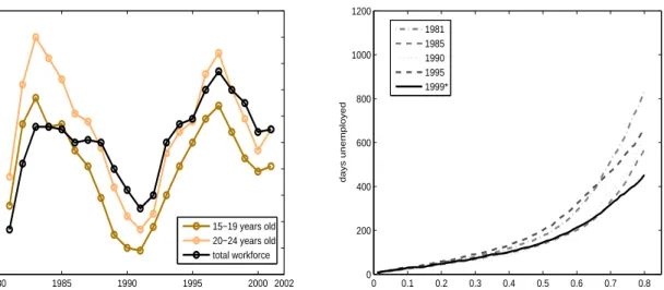
unemploy-ment rates are shown in figure 1 (left graph). It is evident that the unemployunemploy-ment rate of young people in West-Germany decreased relative to the total unemployment rate. Unemployment rates for young people in 1997 (with the highest unemployment rate ever in Germany) were below the maximum numbers during the 1980s. The years 1981 and 1990 are similar in terms of the level of unemployment as well as 1985 and 1995. Figure 1 (right graph) presents nonparametric estimates of the quantile functions in the four years of interest and in 1999. In contrast to results on unem-ployment levels, the quantile functions for 1985 and 1990 are almost identical. Surprisingly, 1981 and 1995 are also similar when we ignore the highest quantiles indicating that longer durations are lower in 1995 compared to 1981.18 _{Although the unemployment rate in 1999 was higher than}

17_{Estimating a richer specification showed that age and the educational degree do not have explanatory degree for}

the length of unemployment periods. For this reason they are mostly not considered in the presented estimations.

19804 1985 1990 1995 2000 2002 5 6 7 8 9 10 11 12 13 14 15−19 years old 20−24 years old total workforce 0 0.1 0.2 0.3 0.4 0.5 0.6 0.7 0.8 0 200 400 600 800 1000 1200 quantile days unemployed 1981 1985 1990 1995 1999*

* estimate based on the IABS 1975-2001

Figure 1: Age group specific unemployment rates in West-Germany (Source: IAB Nuremberg) (left); nonparametric unconditional quantile functions for <26 years old (right)

in 1995, the respective quantile function show a reversed different pattern. The quantile function in 1999 is even weakly below the function in 1990 during the economic boom period. Despite the descriptive nature of these findings, it is apparent that total unemployment is not a good predictor of unemployment durations for young workers. The following analysis uses therefore monthly regional unemployment rates which provide more succinct information.

Specifically, we include the following set of covariates for estimation purposes: • gender of the unemployed.

• marital status of the unemployed.

• married females. This variable absorbs possible effects of out of the labor force periods or parental leave periods of females. A child indicator is not used because information about the presence of children is not available for all years.

• married females in the 1990s. This variable accounts for a possible change in the labor force participation rate of the females in the 1990s.

• we use 5 business sector categories: agriculture, trade/services/traffic, construction, public sector, others (mainly production). The variables are grouped according to the similarity of the results in preliminary estimations.

• wage quintile 4,5. This variables indicates whether the unemployed had pre–unemployment earnings in the highest 40% of the population earnings distribution.

• quarterly GDP growth rate. This variable is the quarterly change in gross GDP measured in prices of 1995. It is affected by seasonal variation and by the business cycle in general. • recall dummy indicating a recall to the former employer at the end of the previous

unem-ployment period.

• four categories for regional information: Rhineland-Palatinate/Hesse, Baden-Wuerttemberg, Bavaria and northern states/Saarland (reference group). These categories are also con-structed according to similarity in preliminary estimation results.

• monthly unemployment rate at the state level unemployment office districts which mainly overlap with the areas of the federal states.

• length of tenure before unemployment: less than one year, 1-3 years (reference category), more than 3 years.

• three calender year indicators: 1981 (reference year), 1985, 1990, 1995.

• indicator for no completed apprenticeship in 1995.

• winter time indicator, which is one if the unemployment spell starts between October and March.

Information about the educational degree and age variables are mostly not considered because preliminary estimates did not suggest that these variables have a sizeable effect. A descriptive summary of the sample is presented in table 1 in the appendix. Only about 8% of the unemploy-ment spells are right censored, which is quite a moderate degree of censoring in the context of duration analysis.

3.2

Estimation Results

We estimate a log-linear version of model (1), i.e.

log(Ti) = x0iβθ+²θi,

at each decile, θ = 0.1,0.2, . . . ,0.9. The CQR model is estimated using the BRCENS algorithm implemented in TSP. Inference on the CQR coefficients is based on 500 bootstrap resamples using

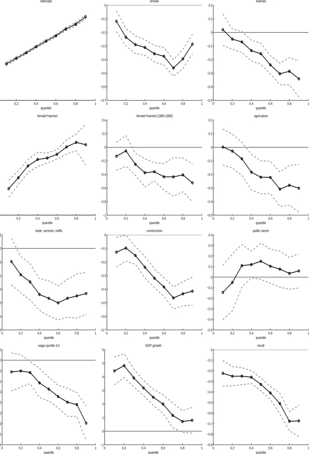
the method of Bilias et al. (2000). The estimations involve the 22 covariates of table 1 and the constant. The estimated coefficients are reported in figures 2 and 3. It is evident that many of them vary significantly over the quantiles. The magnitude or even the sign of the effect of a covariate then differs between short-term (lower quantiles) and long-term unemployed (upper quantiles) indicating the need for a flexible estimation method. For example, the coefficient for the covariate ”married” is not significant for short unemployment duration but its magnitude increases continuously and it is highly negative at the upper quantiles. The winter time variable elongates short duration and shortens long duration. However, the calender time effect has to be considered jointly with the quarterly GDP growth rate, the calender year dummies, and the monthly unemployment rate. For this reason, it is hard to interpret this result. As outlined in the previous section, the Cox-proportional hazard model does not allow for a change of sign of the partial derivative of the conditional quantile function, as observed very clearly for the coefficient of the winter dummy.

Let us now turn to a more detailed discussion of the estimation results and compare them to the results of L¨udemann et al. (2004) for middle aged workers using the same econometric model with different data. Unmarried females exhibit shorter unemployment spells than unmarried males. Married males have shorter unemployment duration than unmarried males. Married females have the longest unemployment duration and the difference to the other groups is very strong. This reflects periods out of the labor force coinciding with parental leave decisions. Unemployment periods of married females became shorter during the 1990s. These results are broadly in line with the findings of L¨udemann et al. (2004). A high level of earnings or a recall to the former employer in the past induce much shorter long term unemployment periods. The regional unemployment rate is not significant at any quantile of the distribution and underpins the findings of L¨udemann et al. (2004) that the unemployment rate does not have an explanatory degree for the length of unemployment periods in Germany. It is observed that unemployment periods in the South German federal states are shorter and in particular long term unemployment periods are much shorter in Bavaria than in the north of Germany. This is in line with the findings of Fahrmeir et al. (2003) and Arntz (2005) who use other samples of unemployed and different estimation techniques. The results for length of tenure suggests that unemployment duration are longer if the foregoing employment spell is short (<1 year) or long (>3 years). Turning to the calender time effect we find that unemployment periods are shorter in 1985 and 1990. Interestingly, they have almost the same length in 1981 and 1995, with the exception that periods of long term unemployment are much shorter in 1995.19 _{This observation coincides with the shape of the}

19_{The highest quantile in 1995 should be read with caution because estimation results may be affected by the}

0 0.2 0.4 0.6 0.8 1 0 1 2 3 4 5 6 7 8 9 intercept quantile 0 0.2 0.4 0.6 0.8 1 −0.7 −0.6 −0.5 −0.4 −0.3 −0.2 −0.1 0 female quantile 0 0.2 0.4 0.6 0.8 1 −0.5 −0.4 −0.3 −0.2 −0.1 0 0.1 0.2 married quantile 0 0.2 0.4 0.6 0.8 1 0 0.2 0.4 0.6 0.8 1 1.2 1.4 1.6 1.8 2 female*married quantile 0 0.2 0.4 0.6 0.8 1 −1 −0.8 −0.6 −0.4 −0.2 0 0.2 0.4 female*married (1990,1995) quantile 0 0.2 0.4 0.6 0.8 1 −0.5 −0.4 −0.3 −0.2 −0.1 0 0.1 0.2 agriculture quantile 0 0.2 0.4 0.6 0.8 1 −0.3 −0.25 −0.2 −0.15 −0.1 −0.05 0 0.05

trade, services, traffic

quantile 0 0.2 0.4 0.6 0.8 1 −0.7 −0.6 −0.5 −0.4 −0.3 −0.2 −0.1 0 construction quantile 0 0.2 0.4 0.6 0.8 1 −0.5 −0.4 −0.3 −0.2 −0.1 0 0.1 0.2 0.3 0.4 public sector quantile 0 0.2 0.4 0.6 0.8 1 −0.4 −0.35 −0.3 −0.25 −0.2 −0.15 −0.1 −0.05 0 0.05 wage quintile 4,5 quantile 0 0.2 0.4 0.6 0.8 1 −1 0 1 2 3 4 5 6 GDP growth quantile 0 0.2 0.4 0.6 0.8 1 −0.9 −0.8 −0.7 −0.6 −0.5 −0.4 −0.3 −0.2 −0.1 0 recall quantile

0 0.2 0.4 0.6 0.8 1 −0.4 −0.35 −0.3 −0.25 −0.2 −0.15 −0.1 −0.05 0 Rhineland−Palatinate, Hesse quantile 0 0.2 0.4 0.6 0.8 1 −0.5 −0.45 −0.4 −0.35 −0.3 −0.25 −0.2 −0.15 −0.1 −0.05 0 Baden−Wuerttemberg quantile 0 0.2 0.4 0.6 0.8 1 −0.7 −0.6 −0.5 −0.4 −0.3 −0.2 −0.1 0 Bavaria quantile 0 0.2 0.4 0.6 0.8 1 −0.04 −0.03 −0.02 −0.01 0 0.01 0.02

monthly regional unemployment rate

quantile 0 0.2 0.4 0.6 0.8 1 −0.1 −0.05 0 0.05 0.1 0.15 0.2 0.25

previous employment duration <1 year

quantile 0 0.2 0.4 0.6 0.8 1 −0.05 0 0.05 0.1 0.15 0.2 0.25 0.3

previous employment duration >3 years

quantile 0 0.2 0.4 0.6 0.8 1 −0.5 −0.45 −0.4 −0.35 −0.3 −0.25 −0.2 −0.15 −0.1 −0.05 0 1985 quantile 0 0.2 0.4 0.6 0.8 1 −0.45 −0.4 −0.35 −0.3 −0.25 −0.2 −0.15 −0.1 −0.05 0 1990 quantile 0 0.2 0.4 0.6 0.8 1 −0.6 −0.5 −0.4 −0.3 −0.2 −0.1 0 0.1 0.2 1995 quantile 0 0.2 0.4 0.6 0.8 1 −0.4 −0.3 −0.2 −0.1 0 0.1 0.2 0.3 winter quantile 0 0.2 0.4 0.6 0.8 1 0 0.1 0.2 0.3 0.4 0.5 0.6 0.7 0.8 no vocational training * 1995 quantile

0 100 200 300 400 500 600 700 800 1 1.5 2 2.5 3 3.5 4 4.5 5 5.5x 10 −3 days unemployed unmarried married 0 100 200 300 400 500 600 700 800 1 1.5 2 2.5 3 3.5 4 4.5 5 5.5x 10 −3 days unemployed summer winter

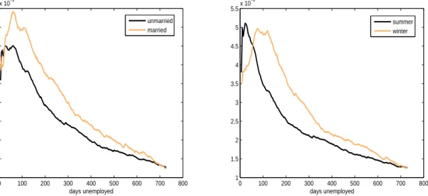
Figure 4: Estimated conditional hazard rates evaluated at sample means of the other regressors. nonparametric quantile functions in figure 1, right. It is maybe related to policy measures against long-term unemployment of young workers that were possibly conducted during this period.

As shown in section 2.3 one can also estimate hazard functions using the GMP resampling procedure. Figure 4 presents different hazard rate estimates based on this methodology. For the reasons provided at the end of section 2.3 we base our hazard rate estimations on nonparametric density estimates for the log duration. The number of resamples is 500. Since almost 10% of our observations are right censored, we draw θm from the uniform distribution on (θl, θu) = (0,0.9). Both plots in figure 4 show that the estimated hazard rates are non–proportional over the duration time. The proportional hazard assumption is apparently violated in this application.20

4

Summary

This survey summarizes recent estimation approaches using quantile regression for (right-censored) duration data. We provide a discussion of the advantages and drawbacks of quantile regression in comparison to popular alternative methods such as the (mixed-)proportional hazard model or the accelerated failure time model. We argue that quantile regression methods are robust and flexible in a sense that they can capture a variety of effects at different quantiles of the duration distribution. Our theoretical considerations suggest that ignoring random effects is likely to have a smaller effect on quantile regression coefficients than on estimated hazard rates of proportional

20_{Note that we have not tested this statistically based on the estimated hazard rates. So far, no formal test}

hazard models. Quantile regression do not impose a proportional effect of the covariates on the hazard. The proportional hazard model is rejected empirically when the estimated quantile regression coefficients change sign across quantiles and we show that this holds even in the presence of unobserved heterogeneity. However, in contrast to the proportional hazard model, quantile regression can not take account of time–varying covariates and it has not been extended so far to allow for unobserved heterogeneity and competing risks. We also discuss and slightly modify the simulation approach for the estimation of hazard rates based on quantile regression coefficients, which has been suggested recently by Machado and Portugal (2002) and Guimar˜aes et al. (2004). Our empirical application to unemployment duration data for young workers from West Ger-many demonstrates the usefulness of the discussed methods. Many estimated coefficients vary over the quantiles of the duration distribution and we observe changes of their sign. Competing alternative estimation approaches, such as a proportional hazard rate model with time–invariant covariates, cannot capture all these effects. Using data for workers aged 26–41, L¨udemann et al. (2004) observe similar violations of the proportional hazard assumption. Wilke (2005) observes crossings of the survivor functions. We conclude that the proportional hazard rate assumption is not justified in standard analysis of unemployment duration in Germany based on time–invariant covariates. Moreover, we present estimated conditional hazard rates based on quantile regression coefficients. These figures also suggest that the proportional hazard assumption is violated in our application. Our findings illustrate the usefulness of quantile regression for duration analysis.

References

Arntz, M. (2005). The geographical mobility of unemployed workers. Evidence from West-Germany. ZEW Discussion Paper 05-34.

Bender, S., Haas, A., and Klose, C. (2000). The IAB Employment Subsample 1975–1995.

Schmollers Jahrbuch, Vol. 120, 649–662.

Bender, S., Hilzendegen, J., Rohwer, G., and Rudolph, H. (1996). Die IAB–Besch¨aftigtenstichprobe 1975–1990. Beitr¨age zur Arbeitsmarkt– und Berufsforschung. No. 197, Institut f¨ur Arbeitsmarkt-und Berufsforschung der BArbeitsmarkt-undesanstalt f¨ur Arbeit (IAB) N¨urnberg.

Biewen, M. and Wilke, R.A. (2005). Unemployment duration and the length of entitlement periods for unemployment benefits: do the IAB employment subsample and the German Socio-Economic Panel yield the same results? Allgemeines Statistisches Archiv 89(2), 209– 236.