STOCHASTIC VOLATILITY MODELS:
CALIBRATION, PRICING AND HEDGING
by
Warrick Poklewski-Koziell
Programme in Advanced Mathematics of Finance
School of Computational and Applied Mathematics
University of the Witwatersrand,
Private Bag-3, Wits-2050, Johannesburg
South Africa
May 2012
ABSTRACT
Stochastic volatility models have long provided a popular alternative to the
Black-Scholes-Merton framework. They provide, in a self-consistent way, an explanation
for the presence of implied volatility smiles/skews seen in practice. Incorporating
jumps into the stochastic volatility framework gives further freedom to financial
mathematicians to fit both the short and long end of the implied volatility surface.
We present three stochastic volatility models here - the Heston model, the Bates
model and the SVJJ model. The latter two models incorporate jumps in the stock
price process and, in the case of the SVJJ model, jumps in the volatility process. We
analyse the effects that the different model parameters have on the implied volatility
surface as well as the returns distribution. We also present pricing techniques for
determining vanilla European option prices under the dynamics of the three models.
These include the fast Fourier transform (FFT) framework of Carr and Madan as
well as two Monte Carlo pricing methods. Making use of the FFT pricing framework,
we present calibration techniques for fitting the models to option data. Specifically,
we examine the use of the genetic algorithm, adaptive simulated annealing and a
MATLAB optimisation routine for fitting the models to option data via a
least-squares calibration routine. We favour the genetic algorithm and make use of it in
fitting the three models to ALSI and S&P 500 option data. The last section of the
dissertation provides hedging techniques for the models via the calculation of option
price sensitivities. We find that a delta, vega and gamma hedging scheme provides
the best results for the Heston model. The inclusion of jumps in the stock price and
volatility processes, however, worsens the performance of this scheme. MATLAB
ACKNOWLEDGMENTS
I would like to thank my supervisor, Dr. Diane Wilcox, for suggesting a
thor-oughly interesting research topic. Her assistance and guidance with the subject
matter of this dissertation helped me immeasurably. Furthermore, I am very
grate-ful to the National Research Foundation1who provided me with a generous bursary
to aid me in my studies. My family and Heather also provided me with continuous
support and encouragement for which I am extremely grateful.
1The opinions expressed in this document do not necessarily represent those of the National
DECLARATION
I declare that this dissertation is my own, unaided work. It is being submitted for
the Degree of Master of Science in the University of the Witwatersrand,
Johannes-burg. It has not been submitted before for any degree or examination in any other
university.
Warrick Poklewski-Koziell
Contents
Table of Contents v
List of Figures vii
1 Introduction 1
2 Stochastic Volatility Models 5
2.1 The Heston Model . . . 5
2.2 The Bates Model . . . 9
2.3 The Double Jump Stochastic Volatility Model . . . 13
2.4 Price Path Comparisons for the Heston, Bates and SVJJ Models . . . 17
3 Pricing Methods 22 3.1 Call Option Pricing with the Fast Fourier Transform . . . 23
3.1.1 Introductory Definitions . . . 23
3.1.2 The Fourier Transform for ATM and ITM Call Options . . . 24
3.1.3 The Fourier Transform for OTM Call Options . . . 26
3.1.4 Using the Fast Fourier Transform to Find the Call Option Price . . 28
3.1.5 The Fast Fourier Transform Algorithm . . . 29
3.1.6 Characteristic Functions for the Heston, Bates and SVJJ Models . . 30
3.1.7 The Complex Logarithm in the Heston Characteristic Function . . . 32
3.1.8 Drawbacks and Alternatives to the Fast Fourier Transform . . . 33
3.2 Monte Carlo Methods . . . 34
3.2.1 The Itˆo-Taylor Expansion . . . 35
3.2.2 The Euler-Maruyama Simulation Scheme . . . 36
3.2.3 The Exact Simulation Scheme . . . 39
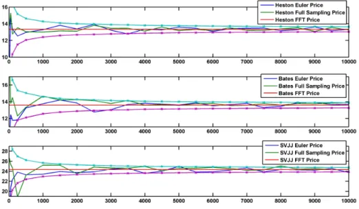
3.3 A Comparison of Pricing Methods . . . 44
3.4 Parallel Monte Carlo Methods for the Heston Model . . . 46
4 Model Calibration 48 4.1 Least-Squares Optimisation . . . 48
4.2 Calibration Methods . . . 50
4.2.1 Global Optimisation with the Genetic Algorithm . . . 50
4.2.2 Global Optimisation with Adaptive Simulated Annealing . . . 58
4.2.3 Local Optimisation with MATLAB lsqnonlin . . . 62
4.3 Calibration Results Using Synthetic Data . . . 63
CONTENTS vi
4.3.1 Calibration of the Heston Model to Synthetic Data . . . 64
4.3.2 Calibration of the Bates Model to Synthetic Data . . . 71
4.3.3 Calibration of the SVJJ Model to Synthetic Data . . . 77
4.3.4 A Summary of Synthetic Data Calibration Results . . . 83
4.4 Calibration Results Using Market Data . . . 83
4.4.1 Calibration to ALSI Options Data . . . 83
4.4.2 Calibration to S&P 500 Options Data . . . 87
4.4.3 A Summary of Market Data Calibration Results . . . 90
4.4.4 A Comment on Calibration Speed Improvements with Parallel Com-puting Methods for the Genetic Algorithm . . . 91
5 Hedging 93 5.1 A Change of Measure in the Heston Model . . . 94
5.2 Hedging Strategies for the Heston Model . . . 97
5.2.1 Delta Hedging in the Heston Model . . . 98
5.2.2 Delta-Sigma Hedging in the Heston Model . . . 98
5.2.3 Delta-Sigma-Gamma Hedging in the Heston Model . . . 99
5.2.4 Simulations of Hedging Methods in the Heston Model . . . 101
5.3 Hedging Strategies for the Bates and SVJJ Models . . . 105
5.3.1 Hedging Simulations for the Bates and SVJJ Models . . . 105
5.3.2 A Comment on Hedging Strategies when Jumps are Involved . . . . 107
6 Conclusion 109 A Risk-Neutral Dynamics for Jump Diffusion Models 111 B Model Characteristic Functions 113 B.1 The Heston Characteristic Function . . . 113
B.2 The Bates Characteristic Function . . . 115
B.3 The SVJJ Characteristic Function . . . 116
C ASAMIN Installation Instructions 117 D Measure Changes for Jump Diffusion Models 118 D.1 A Change of Measure for a Compound Poisson Process as well as a Brownian Motion . . . 118
D.2 A Change of Measure in the Bates Model . . . 120
D.3 A Change of Measure in the SVJJ Model . . . 121
E Selected MATLAB Code 123 E.1 Monte-Carlo Methods . . . 123
E.2 Fast Fourier Transform Pricing Methods . . . 129
E.3 The Genetic Algorithm . . . 140
List of Figures
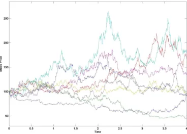
2.1 Sample stock price paths under the Heston model. . . 6
2.2 The effect of ρ on the distribution of stock price returns under the Heston model. . . 7
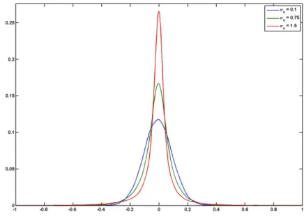
2.3 The effect of σv on the distribution of stock price returns under the Heston model. . . 7
2.4 The effect of ρ andσv on the Heston implied volatility surface. . . 8
2.5 Sample stock price paths under the Bates model. . . 9
2.6 The effect of µS on the distribution of stock price returns under the Bates model. . . 10
2.7 The effect of σS on the distribution of stock price returns under the Bates model. . . 11
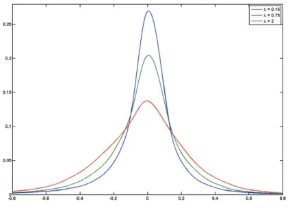
2.8 The effect of λ on the distribution of stock price returns under the Bates model. . . 11
2.9 The effect of µS and σS on the Bates implied volatility surface. . . 12
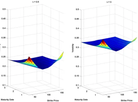
2.10 The effect ofλon the Bates implied volatility surface. . . 12
2.11 Sample stock price paths under the SVJJ model. . . 14
2.12 The effect of ρJ on the distribution of stock price returns under the SVJJ model. . . 15
2.13 The effect of µV on the distribution of stock price returns under the SVJJ model. . . 15
2.14 The effect ofρJ and µV on the SVJJ implied volatility surface. . . 16
2.15 JSE Top 40 index plot. . . 19
2.16 JSE Top 40 daily returns. . . 19
2.17 A comparison between the JSE Top 40 daily returns distribution and the normal distribution. . . 19
2.18 S&P 500 index plot. . . 20
2.19 S&P 500 daily returns. . . 20
2.20 A comparison between the S&P 500 daily returns distribution and the normal distribution. . . 20
2.21 A comparison of stochastic volatility model stock price paths. . . 21
2.22 A comparison of stochastic volatility model volatility paths. . . 21
2.23 A comparison of stochastic volatility model returns. . . 21
3.1 The performance of negative variance value fixes in the Euler-Maruyama scheme for the Heston model. . . 38
LIST OF FIGURES viii
3.2 A comparison of pricing methods for the Heston, Bates and SVJJ models. . 44
4.1 Heston calibration with the GA — Histograms showing the deviation of the calibrated option prices from the original prices. . . 65 4.2 Heston calibration with the GA — Plot of the fittest individual across all
generations. . . 66 4.3 Heston calibration with ASA — Histograms showing the deviation of the
calibrated option prices from the original prices. . . 67 4.4 Heston calibration with ASA — Convergence of the objective function to a
minimum. . . 68 4.5 Heston Calibration with MATLAB lsqnonlin — Histograms showing the
de-viation of the calibrated option prices from the original prices. . . 69 4.6 Heston Calibration with MATLAB lsqnonlin — Convergence of the objective
function to a minimum. . . 70 4.7 Heston Calibration with MATLAB lsqnonlin — Histograms showing the
de-viation of the calibrated option prices from the original prices (with κ fixed). 70 4.8 Bates calibration with the GA — Histograms showing the deviation of the
calibrated option prices from the original prices. . . 72 4.9 Bates calibration with the GA — Plot of the fittest individual across all
generations. . . 72 4.10 Bates calibration with ASA — Histograms showing the deviation of the
cal-ibrated option prices from the original prices. . . 73 4.11 Bates Calibration with MATLAB lsqnonlin — Histograms showing the
devi-ation of the calibrated option prices from the original prices. . . 75 4.12 Bates Calibration with MATLAB lsqnonlin — Convergence of the objective
function to a minimum. . . 76 4.13 Bates Calibration with MATLAB lsqnonlin — Histograms showing the
devi-ation of the calibrated option prices from the original prices (with κ fixed). 76 4.14 SVJJ calibration with the GA — Histograms showing the deviation of the
calibrated option prices from the original prices. . . 78 4.15 SVJJ calibration with the GA — Plot of the fittest individual across all
generations. . . 78 4.16 SVJJ calibration with ASA — Histograms showing the deviation of the
cal-ibrated option prices from the original prices. . . 80 4.17 SVJJ Calibration with MATLAB lsqnonlin — Histograms showing the
devi-ation of the calibrated option prices from the original prices. . . 81 4.18 SVJJ Calibration with MATLAB lsqnonlin — Convergence of the objective
function to a minimum. . . 82 4.19 SVJJ Calibration with MATLAB lsqnonlin — Histograms showing the
devi-ation of the calibrated option prices from the original prices (with κ fixed). 82 4.20 ALSI options calibration — Deviation of calibrated model prices from market
prices. . . 85 4.21 ALSI options calibration — Heston fit to ALSI implied volatility skews. . . 85 4.22 ALSI options calibration — Bates fit to ALSI implied volatility skews. . . . 86 4.23 ALSI options calibration — SVJJ fit to ALSI implied volatility skews. . . . 86
LIST OF FIGURES ix
4.24 S&P 500 options calibration — Deviation of calibrated model prices from market prices. . . 88 4.25 S&P 500 options calibration — Heston fit to S&P 500 implied volatility skews. 88 4.26 S&P 500 options calibration — Bates fit to S&P 500 implied volatility skews. 89 4.27 S&P 500 options calibration — SVJJ fit to S&P 500 implied volatility skews. 89
5.1 Performance of the delta hedging scheme in the Heston model. . . 102 5.2 Performance of the delta-sigma hedging scheme in the Heston model. . . 103 5.3 Performance of the delta-sigma-gamma hedging scheme in the Heston model. 104 5.4 A comparison of hedging schemes in the Heston model. . . 104 5.5 A comparison of hedging schemes in the Bates model. . . 106 5.6 A comparison of hedging schemes in the SVJJ model. . . 106
Chapter 1
Introduction
Financial mathematicians continuously seek to find stock price models that best explain observed stock price dynamics. The most influential of these models has been the Black-Scholes-Merton model (Black and Scholes [7]; Merton [42]) that was formulated in the early 1970’s by the three men after whom the model is named. Much of the popularity of the model came about as a result of its simplicity and the ease with which it provides pricing and hedging solutions for option contracts. This simplicity, however, has many drawbacks. Notably, the model enforces constant stock volatilities and permits only log-normally distributed asset returns. Such dynamics have been shown to be inconsistent with observations in actual financial markets. Market crashes have occurred far more frequently than anticipated by these dynamics. One of the most notable crashes was that of 1987, which led to the emergence of higher implied volatilities for in and out-of-the-money options than at-the-money options. This was due to an increased awareness that the model was incapable of describing the tail activities of stock price probability distributions. Such observations have lead some financial experts to investigate certain stylised facts in financial markets — that stock returns exhibit excess kurtosis and skewness, that volatility is non-constant and tends to cluster and, increasingly, that many markets show signs of jumps in stock prices (and even in the stock price volatility). This has lead to the exploration of stock price models that exhibit such characteristics.
In the past two decades, much research has centred around incorporating stochastic volatility as well as jump components into stock price models. Works by Bakshi et al. [3], Bates [5], Broadie et al. [10], Duffie et al. [22], Gatheral [25] and Heston [28] — to name but a few — have explored the merits and hindrances of using such models to explain stock price dynamics. These models are complex and do not always yield closed form solutions for option pricing. They are, however, very useful in allowing mathematicians to fit both
2
the short and long end of the implied volatility surface. They give a realistic explanation for the presence of the implied volatility skew and are more robust in their descriptions of stock price and volatility movements than the Black-Scholes model is.
In this dissertation, we examine three stochastic volatility models, namely the Heston model, the Bates model and a stochastic volatility model with jumps in both the stock price and variance processes (SVJJ model). Each model is an extension of the previous one, starting with the Heston model, which comprises a stock price process similar to that of the Black-Scholes price process, where the constant volatility term has been replaced by a stochastic term evolving according to a mean-reverting diffusion process. The Bates model then allows for the inclusion of a jump term in the stock price process, while the SVJJ model also includes a jump term in the volatility process. Heston [28] saw the need to devise a stochastic volatility model capable of explaining the skewness in the distributions of stock price returns, as well as the empirically observed implied volatility skew. At the same time, he desired a model that exhibited a “closed-form” (i.e. an integral representation) method for pricing vanilla European options and appealed to Fourier transform techniques for this purpose. This led to the formulation of the Heston model, which today is still extremely popular due to its ability to replicate many observed market phenomena, as well as the ease with which vanilla option prices can be computed under the dynamics of the model. Bates [5] extended this model due to his observation that it was unable to fully explain the implied volatility smile resulting from excess kurtosis in returns distributions. He argued that adding jumps to the price process of the model made it more capable of this task and thus more empirically consistent. In his analysis, he tested his model on Deutsche Mark options data over the period 1984 to 1991 and found evidence supporting the need for jumps in the stock price process of the model.
The paper by Duffie et al. [22] provides a comprehensive treatment on affine jump-diffusion processes. A model that arises naturally from their analysis is the SVJJ model and they compare the performance of this model to the Bates and the Heston models. Calibrating the three models to option data, the authors find that the SVJJ model provides the best fit to the data. Other works of particular interest to us are those by Bakshi et al. [3], Broadie et al. [10] and Gatheral [25]. All three give insight into the addition of jump terms to the stock price and variance processes and find, to varying degrees, that the inclusion of jumps is necessary for stochastic volatility models to comply with market observed phenomena.
The rest of this dissertation is structured as follows. In Chapter 2, we review the three stochastic volatility models and show some of the effects that the models’ parameters have on
3
stock price returns as well as on the implied volatility surface. Chapter 3 considers pricing methods for the three models. More specifically, we examine the application of the fast Fourier transform to vanilla European option pricing under these models. The framework that we follow is that laid out by Carr and Madan [13]. We also consider the paper by Broadie and Kaya [11], which provides a detailed analysis of two Monte Carlo methods that can be applied to the models. Chapter 4 examines the calibration of the models to synthetic as well as to market data. Specifically, we calibrate the models to option price data from the South African All Share Index (ALSI) as well as the S&P 500 index. Options on the ALSI are futures options and so our modelling of these options in a stochastic volatility setting amounts to assuming that the dynamics of the underlying forward price are described by one of the three stochastic volatility models analysed in this dissertation. In this chapter, we compare three calibration methods based on three optimisation routines, namely the genetic algorithm, adaptive simulated annealing and a non-linear least squares method, lsqnonlin, available with the MATLAB software. Finally, chapter 5 examines hedging methods that can be applied to vanilla call options whose underlying assets follow the dynamics of the Heston, Bates and SVJJ models. Specifically, we focus on hedging methods using option price sensitivities to the underlying parameters. Such an analysis would also be useful in the setting of hedging methods for exotic options.
The purpose of this document is to provide a thorough overview of the three models and pricing, calibration and hedging techniques that can be used to implement the models in practical settings. As such, the dissertation is aimed more at practitioners than mathemati-cians and a major emphasis of the work is on the numerical implementation of the numerous techniques. We intend that the subject matter contained here will give readers a good un-derstanding of the dynamics of the different models as well as a consistent framework for approaching the core issues behind the implementation of these models
MATLAB was used extensively as a means of simulating the pricing, calibration and hedging routines presented in this dissertation. Some of the code for these routines is pre-sented in the appendix. All results were obtained via implementation of code in MATLAB 2010b (running in Microsoft Windows 7), on a desktop supercomputer incorporating an Intel Core i7-970 3.2GHz hexacore CPU, 24GB DDR3 RAM and a C2050 Tesla GPU.
Finally, it is important to note some topics that are beyond the scope of this dissertation. Investigations into these topics in further research reports would provide valuable extensions to our work. We have not considered no-arbitrage bounds for the market implied volatility surfaces in this project. In practice, these are very important to ensure that the calibrated
4
surfaces are free from arbitrage. Such bounds are usually set up to ensure that call spreads, butterfly spreads and calendar spreads cannot be constructed off the surfaces to produce arbitrage strategies. An extension of the subject matter in Chapter 4 would be to explore the literature on such no-arbitrage bounds and thus further the investigation into calibrat-ing stochastic volatility models to South African implied volatility data. A particularly useful paper for such an investigation is by Carr and Madan [14]. Moreover, we have not considered the temporal stability of option price parameters, nor have we considered the fitting of models to historical data on the underlying asset. Instead, we have examined the calibration of stochastic volatility models to implied volatility surfaces at single points in time. Obviously, this only gives us an idea of the (risk-neutral) dynamics of the underlying asset process at that time. A valuable extension to this approach would be to evaluate how model parameters change over time and to examine risk premia in the market. Lastly, we have not explored other methods for dealing with non-constant volatility. Such alternatives include local volatility models (see, for example, Gatheral [25]) and GARCH type models (see, for example, Pakel et al. [46]). These alternatives are explored extensively in the finan-cial mathematics literature and provide different approaches for dealing with the volatility surface in option markets.
Chapter 2
Stochastic Volatility Models
2.1
The Heston Model
The Heston model was introduced in the 1993 paper by Steven Heston [28]. The model specifies the following risk-neutral stock price dynamics:
dSt = rStdt+ p VtStdWf (1) t (2.1) dVt = κ(θ−Vt)dt+σv p VtdWf (2) t (2.2) dfW (1) t dWf (2) t = ρdt, (2.3)
wherer is the risk-neutral rate of return, andWf
(1)
t andWf
(2)
t are two correlated Brownian motions under the risk-neutral measure. Here we consider only the risk-neutral dynamics of the stock price process. In chapter 5, we will explore the existence of equivalent martingale measures and examine the transformation from real-world dynamics to those under the risk-neutral measure. From the specification above, we can see that the Heston model is a pure diffusion model — it does not permit jumps in the stock price or the variance processes. The stock price process is similar to that specified under the Black-Scholes model. Here, however, the constant volatility term that appears in the Black-Scholes model has been replaced by a stochastic one which follows the same mean-reverting square root process used by Cox et al. [21] in their famous interest rate model. Figure 2.1 gives an example of ten Heston stock price paths.
The main parameters of interest in the Heston Model areκ,ρ andσv. The rate at which the variance process reverts to its long run average θ is given by the parameter κ. High values ofκessentially turn the stochastic volatility into a time dependent deterministic one, since any deviations in the variance fromθ are immediately pulled back. The parameter ρ
affects the skewness of the returns distribution (see Figure 2.2) and hence the skewness in 5
2.1 The Heston Model 6
the implied volatility smile. Negative values ofρ induce a negative skewness in the returns distribution since lower returns will be accompanied by higher volatility which will stretch the left tail of the distribution. The reverse is true for positive correlation. The parameter
σv affects the kurtosis of the returns distribution and hence the steepness of the implied volatility smile (see Figure 2.3). Large values of σv cause more fluctuation in the volatility process (provided κis not too large) and hence stretch the tails of the returns distribution in both directions. Figure 2.4 shows the effects thatρand σv have on the implied volatility surface.
Figure 2.1Sample Heston stock price paths forS0 = 100,κ= 1.5,θ=V0 = 0.04,
σv = 0.2,ρ= 0.8. The plot was produced using Euler Monte Carlo methods with 1000 time steps.
2.1 The Heston Model 7
Figure 2.2 The effect of ρ on the distribution of stock price returns under the Heston model. The plot was produced using Euler Monte Carlo methods with 100,000 paths and 100 time steps. We can see how negative values of ρ induce negative skewness in the stock price returns distribution and vice versa.
Figure 2.3 The effect of σv on the distribution of stock price returns under the Heston model. The plot was produced using Euler Monte Carlo methods with 100,000 paths and 100 time steps. We can see how larger values of σv increase the kurtosis in the returns distribution.
2.1 The Heston Model 8
Figure 2.4 The effect ofρ and σv on the Heston implied volatility surface. The figure was produced using FFT pricing techniques. The top three plots show how the skewness in the volatility surface changes for positive and negative values of
ρ. The bottom three plots show how the steepness increases for increasing values of σv.
2.2 The Bates Model 9
2.2
The Bates Model
The Bates model was introduced by David Bates [5] in his 1996 paper and is an extension of the Heston model to include jumps in the stock price process. The model has the following risk-neutral dynamics defining the evolution of St:
dSt = (r−λµJ)Stdt+ p VtStdWf (1) t +J StdNet (2.4) dVt = κ(θ−Vt)dt+σv p VtdfW (2) t (2.5) dWf (1) t dfW (2) t = ρdt. (2.6)
Appendix A gives some intuition for the form of the above stock price process. The
Figure 2.5 Sample Bates stock price paths forS0 = 100, κ= 1.5,θ=V0 = 0.04,
σv = 0.2, ρ= 0.8, λ= 3, µS =−0.05, σS = 0.0001. The plot was produced using Euler Monte Carlo methods with 1000 time steps.
volatility process Vt is the same as that in the Heston model and the driving Brownian motions in the two processes have an instantaneous correlation equal to ρ. The process Net
represents a Poisson process under the risk neutral measure, with jump intensity λ. It is independent of the two Brownian motions in the stock price and variance processes. The percentage jump size of the stock price is dictated by the random variable J, with
1 +J ∼ log-normal µS, σS2
,
where the relationship between µS and µJ is given by
µJ = exp µS+ σS2 2 −1.
Figure 2.5 gives an example of ten Bates stock price paths. It is apparent that adding a jump term to the stock price process produces more volatile price movements than those displayed by the Heston model.
2.2 The Bates Model 10
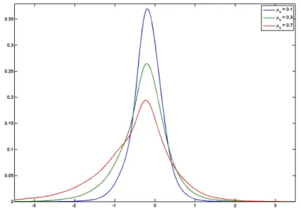
Since the Bates model is an extension of the Heston model, the parameters κ,ρ and σv have the same effect on the returns distribution and implied volatility surface as they do in the Heston model. In addition to these, the parameters defining the jump term in the stock-price process are of particular interest. The parameter µS influences the skewness of the stock price returns distribution, as can be seen in Figure 2.6. Positive values ofµS lead to a positive skew in the distribution of returns. Negative values of µS have the opposite effect. The parameterσS affects the kurtosis of the stock price returns distribution. Larger values ofσS increase the variance of stock price jump sizes and hence increase the kurtosis of the returns distribution. The effect of σS on the returns distribution can be seen in Figure 2.7. The Poisson process intensity parameterλdictates how frequently jumps occur and its effect on the distribution of stock price returns can be seen in Figure 2.8. Larger values of λ increase the occurrence of jumps in the stock price process and this raises the overall level of volatility in the stock price. As a result,λaffects the kurtosis in the returns distribution. Figures 2.9 and 2.10 show the effects that µS, σS and λ have on the implied volatility surface. Note, specifically, how the jump parameters influence the short end of the skew more than they influence the long end. This is one of the advantages of including jumps in a stock price model — the jump terms allow for more flexibility in fitting the short end of the skew. Combining jumps and stochastic volatility makes it easier to fit both the long and short end of the skew.
Figure 2.6 The effect of µS on the distribution of stock price returns under the Bates model. The plot was produced using Euler Monte Carlo methods with 100,000 paths and 100 time steps. The plot demonstrates how negative values of
µS produce negative skewness in the returns distributions under the Bates model. The reverse holds for positive values of µS.
2.2 The Bates Model 11
Figure 2.7 The effect of σS on the distribution of stock price returns under the Bates model. The plot was produced using Euler Monte Carlo methods with 100,000 paths and 100 time steps. We can see how larger values of the parameter increase the kurtosis in the returns distribution.
Figure 2.8 The effect of λ on the distribution of stock price returns under the Bates model. The plot was produced using Euler Monte Carlo methods with 100,000 paths and 100 time steps. It shows that larger values of λ yield more kurtosis in the returns distribution.
2.2 The Bates Model 12
Figure 2.9 The effect of µS and σS on the Bates implied volatility surface. The figure was produced using the FFT pricing framework. The top three plots show how the skewness in the volatility surface changes for positive and negative values of µS. The bottom three plots show how the steepness increases for increasing values of σS.
Figure 2.10 The effect of λ on the Bates implied volatility surface. The figure was produced using the FFT pricing framework. The plots show how the level of volatility increases as λincreases.
2.3 The Double Jump Stochastic Volatility Model 13
2.3
The Double Jump Stochastic Volatility Model
A natural extension of the Bates model is to include jumps in the volatility process in addition to those in the stock price process. Intuitively, it makes sense that a jump in the stock price process should trigger a correlated jump in the volatility process in that sudden, large movements in the stock price would cause increased market anxiety around that stock. As a result, we review the double jump stochastic volatility model (SVJJ) in this subsection.
Works by Broadie et al. (BCJ) [10]; Broadie and Kaya (BK) [11]; Duffie et al. (DPS) [22] and Gatheral [25] all review this model. In particular, the works by BCJ and Gatheral explore the merits and drawbacks of the SVJJ model over Bates-style models. BCJ argue in favour of a stochastic volatility model that incorporates jumps in both the stock price and variance processes, while Gatheral finds that a stochastic volatility model with jumps in the stock price process only produces the best fit to the implied volatility surface. In their analysis, BCJ use option futures data on the S&P 500 over the period from 1987 to 2003, a much longer period than many of the other empirical studies of this kind. They argue that since jumps occur relatively infrequently in stocks, it is wise to use an extended period of observation in order to reduce bias in the data. They also propose that any jump in the stock price should trigger a simultaneous jump in the underlying volatility process. The model that they consequently advocate is the SVCJ model — a stochastic volatility model with contemporaneous jumps in the stock price and its volatility. Notably, the simple stochastic volatility model (Heston) and the stochastic volatility model with jumps in the stock price process only (Bates) are specific cases of this model.
In our formulation of the SVJJ model, we follow the framework by DPS [22] closely. This model has the following risk-neutral dynamics1:
dSt = (r−λµJ)Stdt+ p VtStdWf (1) t +J StdNet (2.7) dVt = κ(θ−Vt)dt+σv p VtdfW (2) t +ZdNet (2.8) dWf (1) t dfW (2) t = ρdt. (2.9)
Again,Netrepresents a Poisson process under the risk neutral measure, with jump intensity
λ. The jump terms in the model are defined as follows:
Z ∼ Exponential (µV)
(1 +J)|Z ∼ log-normal µS+ρJZ, σ2S
,
1
See Appendix A for an explanation of the form of the stock price process in jump-diffusion models under risk-neutral dynamics.
2.3 The Double Jump Stochastic Volatility Model 14
Figure 2.11 Sample SVJJ stock price paths forS0 = 100,κ= 1.5,θ=V0 = 0.04,
σv = 0.2, ρ = 0.8,λ = 3, µS = −0.05, σS = 0.0001, ρJ = −0.4, µV = 0.01. The plot was produced using Euler Monte Carlo methods with 1000 time steps.
where µJ = expnµS+ σ2 S 2 o 1−ρJµV −1.
Figure 2.11 gives an example of ten paths produced using the SVJJ model. These paths exhibit even more volatility than that displayed by the Bates stock paths.
The parameters of interest in this model areρJ and µV, since the other eight parameters are the same as those in the previous models. The parameterρJ impacts on the skewness of the returns distribution in much the same way thatρ does. The effects of ρJ are, however, more prevalent in the short term. Positive values for the parameter will cause jumps in the volatility process to augment those in the stock price process, inducing a positive skew in stock price returns distributions. The reverse will occur for negative values of ρJ. This is displayed by Figure 2.12. The effects of µV on the stock price returns distribution are seen in Figure 2.13. Since µV affects the size of the jumps in the volatility process, larger values for the parameter raise the level of volatility in the stock price. This also increases the kurtosis of the returns distribution. Figure 2.14 shows how the parameters ρJ and µV impact on the SVJJ implied volatility surface.
2.3 The Double Jump Stochastic Volatility Model 15
Figure 2.12 The effect of ρJ on the distribution of stock price returns under the SVJJ model. The plot was produced using Euler Monte Carlo methods with 100,000 paths and 100 time steps. In a similar way to the parameter ρ — the effects of which are shown under the Heston model subsection in this chapter —
ρJ can be seen to influence the skewness of the returns distribution.
Figure 2.13 The effect of µV on the distribution of stock price returns under the SVJJ model. The plot was produced using Euler Monte Carlo methods with 100,000 paths and 100 time steps. Larger values ofµV clearly increase the kurtosis in the returns distribution.
2.3 The Double Jump Stochastic Volatility Model 16
Figure 2.14The effect ofρJ andµV on the SVJJ implied volatility surface. The figure was produced using the FFT pricing methodology. The top three plots show how the skewness in the volatility surface changes for positive and negative values ofρJ. The bottom three plots show how the steepness and level of volatility increase for increasing values of µV.
2.4 Price Path Comparisons for the Heston, Bates and SVJJ Models 17
2.4
Price Path Comparisons for the Heston, Bates and SVJJ
Models
In this section, we compare the three models considered above and examine JSE Top 40 and S&P 500 index data in our consideration of the merits and drawbacks of the different models. Figure 2.21 gives a comparison of stock price paths for the different models2. To give a meaningful comparison, we have ensured that the same random numbers and same jump times are used to generate all the paths. The most striking aspect of the plot is how the inclusion of jumps increases the potential for large stock price movements. The Bates model paths, and even more so, the SVJJ model paths jump at numerous points in the 4 year time horizon. This allows for large rises and drops in the stock price over small intervals in time. The Heston model, on the other hand produces a much more subdued price path than the other two models produce. Thus, the Bates and SVJJ models are able to generate returns distributions with more skewness and more kurtosis than those produced by the Heston model. This is especially true in the short term. The exclusion of jumps from the Heston model clearly limits the price movements that can be generated by the model.
The plot of the JSE Top 40 index as well as that of the S&P 500 index (Figures 2.15 and 2.18) both give evidence of large movements, as well as jumps in the index values. Notably, the market crash of 1987 is highlighted by the sharp drop in the index value in Figure 2.18. Such movements might quite possibly be modelled by the presence of jumps in the process driving the index value. The plot of the S&P 500 index also shows that there was a large decline in the value of the index between 2000 and 2003 and both index plots highlight the recent market crash. Particularly, we see rapid declines in both indices around the middle of 2008. At other times, the index plots hint at relatively calm market behaviour, with few large value movements. Stochastic volatility models that incorporate jump processes can capture these characteristics by allowing for periods of market stability and also periods of instability characterised by large movements and even jumps in stock prices. We can see such price movements in the Bates and SVJJ stock paths in Figure 2.21.
Looking further at the volatility processes of the different models, displayed in Figure 2.22, we see that the Heston and the Bates models produce identical movements in the stock price volatility. The SVJJ model, on the other hand, allows for jumps in the volatility process and this induces large, sudden movements in the process. All three plots also illustrate that high volatility values and low volatility values tend to cluster together. Specifically, the
2
Note that the parameters chosen to produce these plots are based on reasonable results observed in the literature on such models. Different parameters would yield different plots to the ones observed here.
2.4 Price Path Comparisons for the Heston, Bates and SVJJ Models 18
SVJJ volatility path demonstrates that when a jump is experienced, the level of volatility remains high for a while, before reverting to a mean level. This induces the clustering effect seen in the return time series plots for the models (Figure 2.23). Such characteristics can also be observed in Figures 2.16 and 2.19, induced by periods of high and low market volatility. The Black-Scholes model, conversely, does not exhibit any of these features. This illustrates, to an extent, the inability of the Black-Scholes model to produce empirically consistent stock price movements and returns distributions and gives credence to the use of stochastic volatility models, rather than the Black-Scholes model, in modeling stock price dynamics.
We have also seen the ability of the three stochastic volatility models to produce re-turns distributions which are skewed and have excess kurtosis. The Black-Scholes model, on the other hand, is only capable of producing returns which are normally distributed. Considering Figures 2.17 and 2.20, it is clear that the returns on these two indices are not normally distributed. Rather, they both seem to give evidence of distributions that are slightly negatively skewed and which have fat tails.
All these observations indicate that stochastic volatility models are far more capable of replicating market dynamics than the Black-Scholes model is able to. The inclusion of stochastic volatility and jumps in stock price models is justified by market phenomena such as volatility clustering and market crashes. It consequently seems natural that the topic of stochastic volatility and jumps should be explored further for pricing and hedging purposes. Specifically in less liquid markets, such as exotic options markets, it seems that it would be wise to use such models to obtain more reliable prices and better hedging strategies. It is largely these observations, as well as numerous empirical studies (Bakshi et al. [3], Bates [5], Broadie et al. [10], Duffie et al. [22], Gatheral [25], Heston [28]) of stochastic volatility and jumps in the price and volatility paths of stocks that has sparked our interest in this topic.
2.4 Price Path Comparisons for the Heston, Bates and SVJJ Models 19
Figure 2.15 JSE Top 40 in-dex (TOPI) plot between 1 January 2000 and 31 Decem-ber 2009. In the plot, we have set the starting value of the index to 100. The plot gives evidence of large price move-ments, particularly from 2008 onwards.
Figure 2.16 Daily returns corresponding to the JSE Top 40 index plot above. Evidence of volatility clustering is evi-dent in the plot. The plot also shows a number of jumps in stock price returns and a large amount of volatility around the 2008 market crash. Such characteristics can be cap-tured by stochastic volatility and jump processes.
Figure 2.17 Comparison of the distribution of daily re-turns on the JSE Top 40 in-dex and the normal distribu-tion. We see here that the dis-tribution of returns on the in-dex has fatter tails and a taller peak than the normal tion has. The returns distribu-tion also seems to be slightly negatively skewed.
2.4 Price Path Comparisons for the Heston, Bates and SVJJ Models 20
Figure 2.18 S&P 500 index plot between 1 January 1987 and 31 December 2010. In the plot, we have set the starting value of the index to 100. The plot gives evidence of large price movements, possibly due to the effects of stochastic volatility and jumps.
Figure 2.19 Daily returns corresponding to the S&P 500 index plot above. We can see evidence of volatility cluster-ing as well as price jumps in the returns distribution. The stock market crashes of 1987 and 2008 stand out in the plot.
Figure 2.20 Comparison of the distribution of daily re-turns on the S&P 500 index and the normal distribution. We see here that the distri-bution of returns on the in-dex has fatter tails and a taller peak than the normal tion has. The returns distribu-tion is also slightly negatively skewed. Such characteristics can be produced by stochastic volatility models.
2.4 Price Path Comparisons for the Heston, Bates and SVJJ Models 21
Figure 2.21 Stock price paths for the Black-Scholes, Heston, Bates and SVJJ models. The same random numbers were used to generate all the paths. Model parameters: κ = 1.5,
θ = V0 = 0.008, σv = 0.2,
ρ =−0.8,λJ = 3, µS =−0.05,
σS = 0.0001, ρJ = −0.4 and
µV = 0.01. The SVJJ and Bates paths exhibit the great-est price movements, while the Heston and Black-Scholes paths are more subdued.
Figure 2.22 Volatility paths corresponding to the above stock price paths. We can clearly see jumps in the SVJJ volatility path, resulting in larger volatility movements than in the Bates and Hes-ton models. The three volatil-ity paths corresponding to the three stochastic volatil-ity models all show signs of volatility clustering. The Black-Scholes volatility path is obviously flat.
Figure 2.23 Returns corre-sponding to the stock price paths above. The SVJJ and Bates paths show evi-dence of jumps in stock re-turns. All three stochas-tic volatility models give signs of volatility clustering. This makes the models more re-alistic than the Black-Scholes model, which exhibits none of these characteristics.
Chapter 3
Pricing Methods
One of the main advantages of the Black-Scholes-Merton framework (Black and Scholes [7]; Merton [42]) is that it allows for the derivation of closed form option pricing formulas for vanilla options as well as many types of exotic options. The models considered in the previous chapter do not provide pricing solutions quite as easily. Many authors (notably Bates [5], Duffie et al. [22] and Heston [28]) have derived integral representations for vanilla European option prices in such situations through the use of partial differential equations and Fourier transform techniques. The use of these solutions, however, often requires the implementation of somewhat complex numerical methods. A number of the more popular methods include the fast Fourier transform (FFT) and direct integration schemes. As an alternative to deriving and implementing closed form pricing techniques, Monte Carlo methods are also very popular and robust tools for finding option prices under the dynamics of stochastic volatility models.
The application of the FFT to option pricing was made popular by Carr and Madan [13] and enables the rapid computation of option prices across a large grid of strikes. The ability of the Carr and Madan method to simultaneously compute prices for numerous options with equally spaced strike prices is one of its major computational advantages.
A review of direct integration methods is given by Gatheral [25] as well as Zhu [59]. A common way of implementing this method is to express the price of (for example) a vanilla call option as
C(S0, K, T) = S0P1−Ke−rTP2,
where, in a similar way to the Black-Scholes formula, P1 and P2 represent the delta and exercise probability of the option respectively. The terms P1 and P2 involve complicated integral expressions which can be computed using numerical integration techniques, such
3.1 Call Option Pricing with the Fast Fourier Transform 23
as the trapezoidal rule, Simpson’s rule or Gaussian quadrature methods. The method of Attari [1] can also be used with direct integration schemes.
Monte Carlo methods are very popular in mathematical finance. They allow for the pric-ing of options by simulatpric-ing stock paths under the risk neutral measure and averagpric-ing the discounted option payoffs produced by the different paths. These methods are particularly useful in the valuation of exotic options, as well as for the computation of option price sensitivities. Their popularity arises largely as a consequence of their ability to simulate stock paths of even the most complicated stock price models. They can provide option pricing and hedging solutions when no closed form alternatives are available. A drawback here, however, is that they are usually much slower than methods such as the FFT. They are also subject to statistical error: a problem that does not plague the FFT method.
We choose to focus specifically on the Carr and Madan FFT pricing method and Monte Carlo methods in the sections that follow. The FFT method by Carr and Madan is very fast and easy to implement and its ability to compute numerous option prices at once makes it useful as a calibration tool.
3.1
The Carr and Madan Fast Fourier Transform Pricing
Framework for Vanilla European Call Options
The application of the FFT to vanilla option pricing gives a method of rapidly computing option prices. This method can be used whenever the characteristic function of the under-lying stock price process can be derived analytically. Consequently, it has great potential for computing real time option prices, where the dynamics of the stock price process are more complex than those of geometric Brownian motion. We follow the method of Carr and Madan [13] in our application of the FFT to vanilla option pricing.
3.1.1 Introductory Definitions
Definition 1(The Fourier Transform). The Fourier transform of a square-integrable func-tion,g(x), is given by:
ˆ
g(u) =
Z ∞
−∞
eiuxg(x)dx. (3.1)
Definition 2 (The Inverse Fourier Transform). The inverse Fourier transform of a square-integrable function, ˆg(u), is given by:
g(x) = 1 2π
Z ∞
−∞
3.1 Call Option Pricing with the Fast Fourier Transform 24
The Fourier transform of the function g(x) is essentially the transformation of the function from the real domain, to the frequency domain, denoted by u. Furthermore, in order to recover the functiong(x) from the Fourier transform, we apply the inverse Fourier transform. Next we look at the Fourier transform of the probability density function of a random variable, which is of particular importance to the implementation of the FFT.
Definition 3(The Characteristic Function). The characteristic function of a random vari-able,XT, is given by:
φXT (u) = E eiuXT = Z ∞ −∞ eiuXTp(X T)dXT, (3.3)
wherep(XT) is the probability density function ofXT at some time T >0.
3.1.2 The Fourier Transform for ATM and ITM Call Options
The first stage of the application of the FFT to call option pricing is to find the Fourier transform of the call pricing function. When evaluating the Fourier transform of this func-tion, we follow one method for in-the-money (ITM) and at-the-money (ATM) options and a slightly different method for out-of-the-money (OTM) options. Suppose that the pricing function of a European call option is given bycT (k). Here, we denote the maturity of the option by T and the log-strike by k. Furthermore, define the price of the underlying stock at the maturity of the option to be ST and let the risk-neutral density ofsT = log (ST) be given by the function pe(sT). Then
cT (k) = Z ∞ k e−rT esT −ek e p(sT)dsT. (3.4) Evaluating the limit as k→ −∞, we see that
lim k→−∞cT(k) = k→−∞lim Z ∞ k e−rT esT −ek e p(sT)dsT = S0.
Consequently, cT (k) does not converge to 0 in the limit and is thus not square-integrable. Since we cannot apply the Fourier transform to a function which is not square-integrable, we need to consider a new call pricing function which is square-integrable. We do this by applying a dampening factor tocT (k) to get
CT(k) := eαkcT (k), (3.5) whereα is a positive constant.
3.1 Call Option Pricing with the Fast Fourier Transform 25
The Fourier transform of CT (k) is given by:
ψT(u) = Z ∞ −∞ eiukCT (k)dk = Z ∞ −∞ e−rTeiukeαk Z ∞ k esT −ek e p(sT)dsTdk = Z ∞ −∞ e−rTpe(sT) Z sT −∞ esT+αk−e(α+1)keiukdkds T (by changing the order of integration)
= Z ∞ −∞ e−rTpe(sT) Z sT −∞ esT+(α+iu)k−e(α+1+iu)kdkds T = Z ∞ −∞ e−rTpe(sT) " eisT(u−(α+1)i) (α+iu) (α+ 1 +iu) # dsT = e −rT (α+iu) (α+ 1 +iu) Z ∞ −∞ ei(u−(α+1)i)sT e p(sT)dsT = e −rTφ sT(u−(α+ 1)i) (α+iu) (α+ 1 +iu) . (3.6)
Here, φsT(·) denotes the characteristic function (under the risk-neutral measure) of the
log-stock price. Now, considering the inverse Fourier transform ofCT (k), we see that
eαkcT (k) = CT(k) = 1 2π Z ∞ −∞ e−iukψT (u)du and hence that
cT (k) = e−αk 2π Z ∞ −∞ e−iukψT (u)du = e −αk π Z ∞ 0 Re h e−iukψT (u) i du. (3.7)
The above holds because Re
e−iukψT (u)
is an even function (See Carr and Madan [13], Lee [39]). Consequently, the price of a European call option is given by
cT (k) = e−αk π Z ∞ 0 Re e−iuke −rTφ sT(u−(α+ 1)i) (α+iu) (α+ 1 +iu) du. (3.8)
Choosing an Appropriate Value for α
We include the factoreαkwhen performing the Fourier transform of our call pricing function to ensure that the consequent modified call pricing function is integrable over negative values of k. Sinceα is positive, however, this factor worsens the integrability of the modified call pricing function over positive values ofk. In order to ensure that the modified call pricing
3.1 Call Option Pricing with the Fast Fourier Transform 26
function is integrable over all values of k, Carr and Madan [13] state that it is sufficient to ensure that the Fourier transform of our modified call pricing function is finite at 0. From equation (3.6), it can be seen that this will be so provided that φsT(−(α+iu)), and
henceEe
STα+1are finite (note that Ee[·] is the expectation operator under the risk-neutral
measure). An upper bound forαcan now be found by considering the analytical expression for the characteristic function. A popular choice for the value ofαis a quarter of this upper bound.
Truncating the Call Pricing Function
In order to calculate option prices from equation (3.8), we need to use numerical methods to compute the integral in that equation. Consequently, we need to truncate the integral in (3.8) at some point a. This will leave us with an approximation forcT (k) given by
ˆ cT (k) = e−αk π Z a 0 Re e−iuke −rTφ sT(u−(α+ 1)i) (α+iu) (α+ 1 +iu) du. (3.9)
Now, the absolute error of this approximation will be
|cT (k)−ˆcT (k)| = e−αk π Z ∞ 0 Re h e−iukψT (u) i du−e −αk π Z a 0 Re h e−iukψT(u) i du = e−αk π Z ∞ a Rehe−iukψT (u) i du .
To minimise this error, we need to choose a value of a large enough so that the value of this integral is small. Carr and Madan [13] show that, for some desired truncation error,,
amust be chosen such that
a > e −αk π √ A ,
where A is a constant chosen such that Ee h
ST(α+1)
i2
≤A. For a more in depth analysis of this method, see Carr and Madan [13] and Pillay [47].
3.1.3 The Fourier Transform for OTM Call Options
The method for evaluating call option prices given by equation (3.8) is effective for ATM and ITM options. When pricing fairly deep OTM call options which are close to maturity, however, the integrand in (3.8) becomes quite oscillatory. This is as a result of such op-tions tending to their intrinsic values as they near maturity (Carr and Madan [13]). As a consequence, Carr and Madan suggest a different approach in the case of OTM options to circumvent this problem. They consider the “time value” of an OTM option.
3.1 Call Option Pricing with the Fast Fourier Transform 27
The time value of an option is equal to the difference between the value of the option and its intrinsic value. Since an OTM option has an intrinsic value of 0, its time value is simply equal to its value. Carr and Madan thus consider a function,zT(k), which takes the value of either a T maturity call or put option (with log-strike k), whichever is out-of-the-money at inception. Defining ζT (u) to be the Fourier transform of zT(k), we can obtain OTM option prices through the application of the inverse Fourier transform given by:
zT (k) = 1 2π Z ∞ −∞ e−iukζT(u)du. (3.10) Now, zT (k) is defined by the following relation (assuming, for simplicity, thatS0 = 1):
zT (k) = e−rT Z ∞ −∞ h ek−esT 1{sT<k,k<0} i e p(sT)dsT +e−rT Z ∞ −∞ h esT −ek 1{sT>k,k>0} i e p(sT)dsT. (3.11) Applying the Fourier transform tozT(k)
ζT (u) = Z ∞ −∞ eiukzT (k)dk = Z ∞ −∞ eiuke−rT Z ∞ −∞ h ek−esT 1{sT<k,k<0} i e p(sT)dsTdk + Z ∞ −∞ eiuke−rT Z ∞ −∞ h esT −ek 1{sT>k,k>0} i e p(sT)dsTdk = Z 0 −∞ eiuke−rT Z k −∞ ek−esT e p(sT)dsTdk + Z ∞ 0 eiuke−rT Z ∞ k esT −ek e p(sT)dsTdk = Z 0 −∞ e−rT Z 0 sT eiuk ek−esT e p(sT)dkdsT + Z ∞ 0 e−rT Z sT 0 eiukesT −ek e p(sT)dkdsT (by changing the order of integration)
= e−rT 1 1 +iu − erT iu − φsT(u−i) u(u−i) . (3.12)
As with the transform for ITM and ATM options, we need to include a dampening factor here. When k = 0 and as T approaches 0, zT (k) becomes quite oscillatory and including the factor sinh (αk) helps to counteract this. The Fourier transform of sinh (αk)zT (k) is given by: γT(u) = Z ∞ −∞ eiuksinh (αk)zT (k)dk = ζT (u−iα)−ζT (u+iα) 2 . (3.13)
3.1 Call Option Pricing with the Fast Fourier Transform 28
Hence, by making use of the inverse Fourier transform, the price of an OTM option is given by: zT(k) = 1 2πsinh (αk) Z ∞ −∞ e−iukγT (u)du = 1 πsinh (αk) Z ∞ 0 Re h e−iukγT (u) i du. (3.14)
3.1.4 Using the Fast Fourier Transform to Find the Call Option Price
In this section, we consider the pricing of ATM and ITM call options using the FFT algo-rithm. The same procedure is followed by Carr and Madan [13] and can easily be extended to the case for OTM call options.
Discretising the integral in the pricing function,
ˆ cT (k) = e−αk π Z a 0 Re h e−iukψT (u) i du,
by using the trapezoidal rule gives us:
ˆ cT(k) ≈ Re e−αk π N X j=1 e−iujkψ T(uj) ∆ , (3.15)
where ∆ gives us the distance between successive points on our discretised integration grid,
uj = ∆ (j−1) and a=N∆.
Now, the FFT is an efficient method of computing the sum
w(v) = N
X
j=1
e−i2Nπ(j−1)(v−1)x(j) (3.16)
for v = 1,2, . . . , N. Consequently, we want to manipulate (3.15) to look like (3.16). This can be achieved by defining
kv = −b+η(v−1), (3.17) whereb= N η2 . Equation (3.17) gives us N log-strike values at regular intervals of width η, ranging from −btob. Finally, settingη∆ = 2πN, we get
ˆ cT (kv) ≈ Re e−αkv π N X j=1 e−iη∆(j−1)(v−1)eibujψ T(uj) ∆ = Re e−αkv π N X j=1 e−i2Nπ(j−1)(v−1)eibujψT (uj) ∆ . (3.18)
3.1 Call Option Pricing with the Fast Fourier Transform 29
Factoring in Simpson’s rule weightings to the above will help to obtain more accurate prices for large values of ∆ (and hence small spaces between successive strike prices). This gives us ˆ cT(kv) = Re e−αkv π N X j=1 e−i2Nπ(j−1)(v−1)eibujψT(uj)∆ 3 3 + (−1)j−1{j=1} , (3.19)
where1 is the indicator function. This is almost identical to equation (3.16), with
x(j) = eibujψ T (uj) ∆ 3 3 + (−1)j −1{j=1} .
Out-of-the-Money Options. For OTM options we have
ˆ cT (k) ≈ 1 πsinh (αk) Z a 0 Rehe−iukγT (u) i du.
Discretising this in a similar way to before, we get
ˆ cT(kv) = Re 1 πsinh (αkv) N X j=1 e−i2Nπ(j−1)(v−1)eibujγT(uj)∆ 3 3 + (−1)j−1{j=1} . (3.20)
3.1.5 The Fast Fourier Transform Algorithm
The power of the FFT (see Zhu [59]) lies in its ability to reduce the number of operations required to compute sums such as those in equations (3.19) and (3.20). ComputingN option prices using either of these would require a number of arithmetical operations of the order of O N2. The FFT, however, drastically reduces this number. Consider the discretised call pricing function for ATM/ITM options given by equation (3.19). We re-write it with
x(j) = eibujψ T (uj) ∆ 3 3 + (−1)j −1{j=1} , to get ˆ cT(kv) = e−αkv π N X j=1 e−i2Nπ(j−1)(v−1)x(j),
where we ignore the use of the operator Re [·] for simplicity. We can now split this sum into two parts by settingM = N2. From Zhu [59]:
ˆ cT(kv) = e−αkv π N 2 X j=1 e−i2Nπ[2(j−1)](v−1)x(2j−1) +e −αkv π N 2 X j=1 e−i2Nπ[2(j−1)+1](v−1)x(2j) = e −αkv π M X j=1 e−i2Mπ(j−1)(v−1)x(2j−1) +e−i 2π N(v−1) M X j=1 e−i2Mπ(j−1)(v−1)x(2j) .
3.1 Call Option Pricing with the Fast Fourier Transform 30
Splitting this into two parts, we see that
ˆ cT (kv) = e−αkv π h ˆ cT(odd)(v) +e−i2Nπ(v−1)ˆc(even) T (v) i (3.21) ifv < M + 1, and ˆ cT(kv) = e−αkv π h ˆ cT(odd)(v−M) +e−i2Nπ(v−1)ˆc(even) T (v−M) i (3.22)
ifv≥M + 1. Now for a given value ofv, sayv∗ where 1≤v∗ ≤M,
h ˆ cT(odd)(v) +e−i2Nπ(v−1)cˆ(even) T (v) i v=v∗ = h ˆ cT(odd)(v−M)−e−i2Nπ(v−1)ˆc(even) T (v−M) i v=v∗+M,
and so we only need to compute the values of 3.21 and we will automatically have those for 3.22. Furthermore, we can break down each of the sub-sequences ˆcT(even)(v) and ˆcT(odd)(v) into two further sub-sequences. Continuing this way, we will eventually arrive at a series of sub-sequences, each of length 1. Ultimately, this allows us to reduce the number of compu-tations required to compute the discretised Fourier transform fromO N2toO(Nlog2N). The reduced number of computations means that the FFT can provide solutions to Fourier transforms much faster than simple summation routines are able to. This is specifically useful when dealing with large values of N.
3.1.6 Characteristic Functions for the Heston, Bates and SVJJ Models
In this subsection, we consider the characteristic functions of the Heston, Bates and SVJJ models. For a more in depth overview of these, see Appendix B.
The Heston Model Characteristic Function
The characteristic function of the log-stock price under the Heston model is given by (Duffie et al. [22], Gatheral [25], Heston [28], Kilin [35]):
φsT (u) = Ee
eiusT
= exp{C(u, T)θ+D(u, T)V0+iu(log (S0) +rT)}, (3.23) where V0 is the initial value of the variance process, T is the expiration date of the option and C(u, T) = κ rnegT− 2 σ2 v log 1−ge−dT 1−g (3.24) D(u, T) = rneg 1−e−dT 1−ge−dT , (3.25)
3.1 Call Option Pricing with the Fast Fourier Transform 31 with g := rneg rpos rpos/neg = β±d 2γ d = pβ2−4αγ α = −u 2−iu 2 β = κ−ρσviu γ = σ 2 v 2 . The Bates Model Characteristic Function
The characteristic function of the log-stock price in the Bates model is the same as that in the Heston model, with the addition of a “jump part”. This gives us (Bates [5], Duffie et al. [22], Gatheral [25], Kilin [35]):
φsT(u) = Ee eiusT = exp{C(u, T)θ+D(u, T)V0+P(u)λT +iu(log (S0) +rT)}, (3.26) where P(u) = −µJiu+ h (1 +µJ)iueσ2S( iu 2)(iu−1)−1 i . (3.27)
The functionsC(u, T) andD(u, T) have the same form as for the Heston model. The SVJJ Model Characteristic Function
The characteristic function of the log-stock price in the SVJJ model is similar to that in the Bates model, however it allows for jumps in both the stock price and variance processes. As a result, we find that the characteristic function of this model has a similar form to that of the Bates model, with a more complicated jump component. This gives us (Duffie et al. [22], Gatheral [25]): φsT(u) = Ee eiusT = exp{C(u, T)θ+D(u, T)V0+P(u, T)λ+iu(log (S0) +rT)}, (3.28) where P(u, T) = −T(1 +iuµJ) + exp iuµS+ σS2(iu)2 2 ν (3.29)
3.1 Call Option Pricing with the Fast Fourier Transform 32 and ν = β+d (β+d)c−2µVα T+ 4µVα (dc)2−(2µVα−βc)2 × log 1−(d−β)c+ 2µVα 2dc 1−e−dT (3.30) c = 1−iuρJµV.
Again,C(u, T) andD(u, T) have the same form as for the Heston model. The expressions forβ,dand α are also the same as in the case for the Heston model.
3.1.7 The Complex Logarithm in the Heston Characteristic Function
Zhu [59] gives a concise overview of the problem with the complex logarithm in the Heston model. He also presents some of the popular methods of solving this issue.
The numerical implementation of Heston’s [28] original formulation of the characteristic function for the model gives rise to numerical instability due to the presence of a complex logarithm. This issue, by extension, also effects the other two models that we are concerned with. Any complex number can be expressed as
z = x+iy
= aeib
= a(cos(b) +isin(b)),
wherea=√a2+b2 and b=b
0+ 2πmsuch that b0∈[−π, π] and m is an integer. Thus,
z = a(cos(b0) +isin(b0)) = aeib0
by Euler’s formula and the properties of sin and cos. Furthermore, the logarithm ofz can be expressed as
log (z) = logaeib
= log (a) +ib
= log (a) +i(b0+ 2πm).
This illustration shows that the complex number, z, is fully and uniquely characterised by a and b0. The logarithm of this number, however, depends on a, b0 and m in such a way that any selected value of m will yield the same value for the complex logarithm.
3.1 Call Option Pricing with the Fast Fourier Transform 33
In general, computational software programs thus set m to zero and consider only the value ofaand b0 — the principal branch — in the computation of a complex number and its logarithm. While this approach is acceptable for individual computations of complex numbers, it causes problems in computations involving the characteristic function of the Heston model. Specifically, it leads to discontinuities in the integrand functions involving the Heston characteristic function in the option pricing expressions for the model. Ignoring these effects can often lead to erroneous option prices.
There are a number of algorithms to take care of this problem, some of which are reviewed by Zhu [59]. In our case, we use a different formulation of the characteristic function of the Heston model to that originally proposed by Heston [28]. This is one which is derived by Gatheral [25] and involves a modification to the complex logarithm in the characteristic function to ensure that it never crosses the negative real axis. This prevents unnecessary branch cuts in the complex logarithm and solves the discontinuity problem. Consequently, it is safe to implement this method without worrying about unwittingly obtaining incorrect option prices.
3.1.8 Drawbacks and Alternatives to the Fast Fourier Transform
The FFT method described above is a fast and efficient method for computing option prices, where the relevant stock price model does not produce a simple closed-form option pricing formula (whereas the Black-Scholes model, for example, does exhibit an easily computable closed-form option pricing formula). This is particularly relevant in our case, where none of the models that we have considered produces such a formula. The ability of the FFT to simultaneously compute option prices for a large range of strikes is also particularly useful. This property greatly reduces computation times for model calibration. The method does, however, have a number of drawbacks and there are alternative pricing methods that can also be used, instead of the FFT method, to find option prices.
One of the major drawbacks of the FFT scheme is that it forces log-strike prices to fall on the grid kv =−b+λ(v−1) (with equally spaced grid points). As a result, the method is limited to pricing only options whose corresponding log-strike prices fall on that grid. To price options with log-strikes that do not fall on the grid requires the use of an appropriate interpolation scheme. Deciding which one to use is not always easy and, regardless of the scheme chosen, some numerical inaccuracy will always result. This can, if not controlled correctly, negatively impact on pricing, calibration and hedging schemes.
3.2 Monte Carlo Methods 34
Another drawback of the FFT method is that the value of N, specifying the number of grid points must always be a power of 2. This is apparent by considering the way in which the FFT algorithm reduces the number of computations required to compute the discretised inverse Fourier transform. This leads to a limitation in the specification of the upper bound of integration for the inverse transform.
A final drawback of the FFT method comes from the relationship λ∆ = 2πN. As a result of this, the size of the spacings in the integration grid, and those in the strike grid are inversely related. If we want to have small spaces between points on the log-strike grid, then we must settle for large spaces between points on the integration grid (or vice versa). This obviously impacts negatively on the accuracy of the method. The inclusion of Simpson’s rule weightings when computing the discrete inverse Fourier transform, as set out in the Carr and Madan [13] option pricing framework, can help to overcome this.
Alternatives to the FFT pricing method include the recently developed COS method by Fang et al. [23], as well as the fractional FFT and direct integration (DI) schemes. Kilin [35] presents an informative comparison of the FFT, fractional FFT and DI schemes. In his paper, he illustrates how an improvement to the FFT method of Carr and Madan — to yield the fractional FFT method — can greatly increase the computational speed of the pricing scheme. He further analyses a caching technique that can be used in conjunction with direct integration schemes to make the computation of option prices for a large range of strikes under the schemes more efficient. He concludes that this final method is the most efficient of the three.
3.2
Monte Carlo Methods
Monte Carlo methods are used extensively in mathematical finance. They provide a con-venient way of simulating stock price distributions and pricing options where closed form solutions are difficult to derive, or do not exist at all. For these reasons, the use of Monte Carlo methods is particularly useful to us. Kloeden and Platen [36] provide a rigorous treatment on the simulation of stochastic differential equations. Of particular interest to us is their derivation of the Itˆo-Taylor expansion in that it forms the basis of the Euler-Maruyama simulation scheme. Gatheral [25] also examines the application of Monte Carlo methods to the simulation of stochastic volatility models. The paper by Broadie and Kaya [11] provides an excellent treatment on exact simulation schemes for the three models with which we are concerned. Such schemes allow for the simulation of stock price processes by sampling from the exact distributions of the stock price and volatility process increments.
3.2 Monte Carlo Methods 35
We also draw from Poklewski-Koziell [48] for our treatment on Monte Carlo methods for the Heston model.
In the sections that follow, we present the Euler-Maruyama and exact simulation schemes for the Heston, Bates and SVJJ models. We also look at the application of these schemes to vanilla call pricing.
3.2.1 The Itˆo-Taylor Expansion
Consider a one dimensional Itˆo stochastic differential equation (SDE) given by (see Kloeden and Platen [36])
dXt = α(Xt)dt+β(Xt)dZt, (3.31) or equivalently in integral form
Xt = X0+ Z t 0 α(Xu)du+ Z t 0 β(Xu)dZu, (3.32) where α(Xt), β(Xt) ∈ C2(<) are stochastic processes adapted to the natural filtration generated by Xt. As usual, Zt is a standard Brownian motion. Next, by applying Itˆo’s Lemma to the function f(Xt)∈C2(<) we get
f(Xt) = f(X0) + Z t 0 L0f(Xu)du+ Z t 0 L1f(Xu)dZu, (3.33) for all t≥0, where
L0 = α ∂ ∂x+ 1 2β 2 ∂2 ∂x2 L1 = β ∂ ∂x.
Now, by applying Itˆo’s Lemma to the processesα(Xt) andβ(Xt), it can shown that equa-tion (3.32) becomes Xt = X0+α(X0) Z t 0 du+β(X0) Z t 0 dZu+R1, (3.34) where the remainder term is defined by
R1 = Z t 0 Z u 0 L0α(Xy)dydu+ Z t 0 Z u 0 L1α(Xy)dZydu + Z t 0 Z u 0 L0β(Xy)dydZu+ Z t 0 Z u 0 L1β(Xy)dZydZu. (3.35)
3.2 Monte Carlo Methods 36
If we do the same forL1β(X
t) in (3.35), we get Xt = X0+α(X0) Z t 0 du+β(X0) Z t 0 dZu +L1β(X0) Z t 0 Z u 0 dZydZu+R2, (3.36) where we define the remainder term
R2 = Z t 0 Z u 0 L0α(Xy)dydu+ Z t 0 Z u 0 L1α(Xy)dZydu + Z t 0 Z u 0 L0β(Xy)dydZu+ Z t 0 Z u 0 Z y 0 L0L1β(Xv)dvdZydZu + Z t 0 Z u 0 Z y 0 L1L1β(Xv)dZvdZydZu. (3.37) The Itˆo-Taylor expansion forms the basis for the derivation of the Euler-Maruyama and one-dimensional Milstein schemes. In what follows, we implement the Euler-Maruyama scheme for the three stochastic volatility models. We choose to implement this method due to its simplicity and speed (relative to other Monte Carlo schemes).
3.2.2 The Euler-Maruyama Simulation Scheme
Euler Monte Carlo for the Heston Model
Truncating equation (3.34) just before the remainder term and applying it to the log-stock price and variance processes of the Heston model yields the Euler-Maruyama scheme for Heston. We consider the log of the stock process and not simply the stock process itself to enforce positive stock price values over all possible simulation paths. Applying Itˆo’s Lemma to the functionf(St) = log (St) yields
dlogSt = rdt− 1 2Vtdt+ p VtdfW (1) t . (3.38)
We can apply the Cholesky decomposition to enforce correlation between the log-stock price and variance processes. This gives us


![Figure 3.1 Comparison of different fixes for the occurrence of negative variance values in Euler-Maruyama simulation scheme for the Heston model (plot taken from Poklewski-Koziell [48]).](https://thumb-us.123doks.com/thumbv2/123dok_us/432412.2549857/47.918.244.739.135.534/comparison-different-occurrence-negative-variance-maruyama-simulation-poklewski.webp)