COMPUTATION OF RADAR CROSS SECTIONS OF COMPLEX TARGETS BY SHOOTING AND BOUNCING RAY METHOD

COMPUTATION OF RADAR CROSS SECTIONS OF COMPLEX TARGETS BY SHOOTING AND BOUNCING RAY METHOD

A THESIS SUBMITTED TO

THE GRADUATE SCHOOL OF NATURAL AND APPLIED SCIENCES OF

MIDDLE EAST TECHNICAL UNIVERSITY

BY

SALİM ÖZGÜN

IN PARTIAL FULFILLMENT OF THE REQUIREMENTS FOR

THE DEGREE OF MASTER OF SCIENCE IN

ELECTRICAL AND ELECTRONICS ENGINEERING

ii

Approval of the thesis:

COMPUTATION OF RADAR CROSS SECTIONS OF COMPLEX TARGETS BY SHOOTING AND BOUNCING RAY METHOD

Submitted by SALİM ÖZGÜN in partial fulfillment of the requirements for the degree of Master of Science in Electrical and Electronics Engineering, Middle East Technical University by,

Prof. Dr. Canan Özgen

Dean, Graduate School of Natural and Applied Sciences ______________

Prof. Dr. İsmet Erkmen

Head of Department, Electrical and Electronics Engineering ______________ Prof. Dr. Mustafa Kuzuoğlu

Supervisor, Electrical and Electronics Engineering, METU ______________

Examining Committee Members:

Prof. Dr. Gönül Turhan Sayan

Electrical and Electronics Engineering, METU ______________ Prof. Dr. Mustafa Kuzuoğlu

Electrical and Electronics Engineering, METU ______________ Prof. Dr. Gülbin Dural

Electrical and Electronics Engineering, METU ______________ Assist. Prof. Dr. Lale Alatan

Electrical and Electronics Engineering, METU ______________

Assist. Prof. Dr. Egemen Yılmaz

Electronics Engineering, Ankara University ______________

iii

I hereby declare that all information in this document has been obtained and presented in accordance with academic rules and ethical conduct. I also declare that, as required by these rules and conduct, I have fully cited and referenced all material and results that are not original to this work.

Name, Last name: Salim Özgün

iv

ABSTRACT

COMPUTATION OF RADAR CROSS SECTIONS OF

COMPLEX TARGETS BY SHOOTING AND BOUNCING

RAY METHOD

Özgün, Salim

M.Sc., Department of Electrical and Electronics Engineering Supervisor: Prof. Dr. Mustafa Kuzuoğlu

August 2009, 66 Pages

In this study, a MATLAB® code based on the Shooting and Bouncing Ray (SBR) algorithm is developed to compute the Radar Cross Section (RCS) of complex targets. SBR is based on ray tracing and combine Geometric Optics (GO) and Physical Optics (PO) approaches to compute the RCS of arbitrary scatterers. The presented algorithm is examined in two parts; the first part addresses a new aperture selection strategy named as “conformal aperture”, which is proposed and formulated to increase the performance of the code outside the specular regions, and the second part is devoted to testing the multiple scattering and shadowing performance of the code. The conformal aperture approach consists of a configuration that gathers all rays bouncing back from the target, and calculates their contribution to RCS. Multiple scattering capability of the algorithm is verified and tested over simple shapes. Ray tracing part of the code is also used as

v

a shadowing algorithm. In the first instance, simple shapes like sphere, plate, cylinder and polyhedron are used to model simple targets. With primitive shapes, complex targets can be modeled up to some degree. Later, patch representation is used to model complex targets accurately. In order to test the whole code over complex targets, a Computer Aided Design (CAD) format known as Stereo Lithography (STL) mesh is used. Targets that are composed in CAD tools are

imported in STL mesh format and handled in the code. Different sweep geometries are defined to compute the RCS of targets with respect to aspect angles. Complex targets are selected according to their RCS characteristics to test the code further. In addition to these, results are compared with PO, Method of Moments (MoM) and Multilevel Fast Multipole Method (MLFMM) results obtained from the FEKO software. These comparisons enabled us to improve the code as possible as it is.

Keywords: Shooting and Bouncing Ray (SBR) Method, Radar Cross Section (RCS), Conformal Aperture, FEKO

vi

ÖZ

KARMA

Ş

IK HEDEFLER

İ

N RADAR KES

İ

T ALANININ

SEKEN I

Ş

IN YÖNTEM

İ

YLE HESAPLANMASI

Özgün, Salim

Yüksek Lisans, Elektrik-Elektronik Mühendisliği Bölümü

Tez Yöneticisi: Prof. Dr. Mustafa Kuzuoğlu

Ağustos 2009, 66 sayfa

Bu çalışmada cisimlerin Radar Kesit Alanının (RKA) hesaplanması için Seken Işın Yöntemi (SIY) algoritması kullanılarak MATLAB® tabanlı bir kod geliştirilmiştir. SIY rastgele seçilmiş hedeflerin RKA değerini hesaplamak için Geometrik Optik (GO) ve Fiziksel Optik (FO) yöntemlerini beraber kullanan ışın takibine dayalı bir algoritmadır. Sunulan algoritma iki bölümde incelenmiştir; ilk bölümde doğrudan yansıma dışında kalan bölgelerde kodun performansını

artırmak için yeni bir yöntem olan “uyumlu açıklık” önerilmiş ve formüle edilmiş, ikinci bölümde ise algoritmanın çoklu yansımaları hesaplama ve gölgeleme performansı test edilmiştir. ”Uyumlu açıklık” yöntemi ile hedeften geri seken

vii

tüm ışınlar toplanıp RKA’ ya katkıları hesaplanmıştır. Algoritmanın çoklu yansıma kabiliyeti sadece basit şekiller üzerinde test edilmiştir. Kodun ışın takibi bölümü aynı zamanda gölgeleme algoritması olarak kullanılmıştır. İlk aşamada basit hedefleri modellemek için küre, plaka, silindir ve polihedron gibi basit

şekiller kullanılmıştır. Ancak basit şekiller ile karmaşık hedefler bir dereceye kadar modellenebilmektedir. Daha sonraki aşamalarda karmaşık şekillerin daha iyi modellenebilmesi için üçgen parçalar kullanılmıştır. Kodu karmaşık hedefler üzerinde test etmek için Bilgisayar Destekli Tasarım (BDT) formatı olan STL ağ

yapısı kullanılmıştır. BDT ortamında modellenen hedefler STL ağ formatında koda taşınmış ve işlem yapılmıştır. Cisimlerin RKA değerlerini bakış açısına göre hesaplayabilmek için farklı döndürme geometrileri kullanılmıştır. Seçilen karmaşık hedeflerde RKA karakteristiklerinin farklı olması göz önünde bulundurulmuştur. Bu çalışmalara ek olarak koddan elde edilen sonuçlar, FEKO yazılımından elde edilen FO, MoM ve MLFMM sonuçları ile karşılaştırılmıştır. Bu karşılaştırma, kodu mümkün olduğunca geliştirme imkânını bize sunmuştur.

Anahtar Sözcükler: Seken Işın Yöntemi (SIY), Radar Kesit Alanı (RKA), Uyumlu Açıklık, FEKO

viii

ix

ACKNOWLEDGEMENTS

I would like to thank my thesis supervisor, Prof. Dr. Mustafa Kuzuoğlu for his guidance, understanding and suggestions. His broad vision and motivation has been a great privilege.

I would also thank my leader Harun Solmaz and age of empires team; Mehmet Karakaş, Selim Kocabay, Mehmetcan Apaydın, Seçkin Arıbal, Aykut Cihangir, Musa Civil, Erdem Kazaklı, Baran Kızıltan and Şükrü Bülent Toker for their great friendship and enjoyable “age of empires the conquerors” times during lunch.

Also, I would like to express my thanks to my family for their understanding and patience.

Lastly, thanks to TAI for supplying the FEKO software and supporting me for this work.

x

TABLE OF CONTENTS

ABSTRACT ... iv ÖZ……… ... vi ACKNOWLEDGEMENTS ... ix TABLE OF CONTENTS ... x

LIST OF TABLES ... xii

LIST OF FIGURES ... xiii

LIST OF FIGURES ... xiii

CHAPTER 1 INTRODUCTION ... 1

1.1 Literature Review ... 3

1.2 Overview of the Thesis ... 4

1.3 Outline of the Thesis ... 5

2 SHOOTING AND BOUNCING RAY METHOD ... 7

2.1 Formulation of the Shooting and Bouncing Ray Method ... 8

2.2 Numerical Results for Simple Targets ... 19

2.3 SBR Final Integration Aperture ... 39

2.4 SBR Multiple Scattering Capability ... 44

2.5 Shadowing ... 46

xi

3.1 Target Modeling ... 49

3.2 Target Rotation ... 52

3.3 Numerical Results ... 53

4 CONCLUSIONS ... 61

4.1 Summary of the Thesis ... 61

4.2 Advantages and Disadvantages of SBR ... 62

4.3 Future Work ... 63

xii

LIST OF TABLES

TABLES

Table 3-1 Computation times for tank model simulation ... 54 

Table 3-2 Computation times for ship model simulation ... 56 

xiii

LIST OF FIGURES

FIGURES

Figure 2.1 SBR, incident rays and exit aperture ... 9 

Figure 2.2 Triangle defined with right hand rule ... 11 

Figure 2.3 A triangle constructed from three half spaces ... 12 

Figure 2.4 Reflection of a ray ... 13 

Figure 2.5 Ray tube ... 16 

Figure 2.6 Shape of exit ray tube ... 18 

Figure 2.7 Simulation setup for monostatic RCS of PEC plate ... 21 

Figure 2.8 Comparison of MoM and SBR results for θθ polarized monostatic RCS of PEC plate with respect to frequency ... 22 

Figure 2.9 Simulation setup for bistatic RCS of PEC plate ... 23 

Figure 2.10 Comparison of MoM and SBR results for θθ polarized bistatic RCS of PEC plate with respect to frequency ... 23 

Figure 2.11 Simulation setup for monostatic RCS of PEC plate ... 24 

Figure 2.12 Comparison of MoM and SBR results for θθ polarized monostatic RCS of PEC plate ... 25 

Figure 2.13 Comparison of PO and SBR results for θθ polarized monostatic RCS of PEC plate ... 26 

Figure 2.14 Simulation setup for bistatic RCS of PEC plate ... 27 

Figure 2.15 Comparison of MoM and SBR results for θθ polarized bistatic RCS of PEC plate ... 28 

Figure 2.16 Simulation setup for bistatic RCS of PEC plate ... 29 

Figure 2.17 Comparison of MoM and SBR results for θθ polarized bistatic RCS of PEC plate with respect to frequency ... 30 

xiv

Figure 2.19 Comparison of PO and SBR results for θθ polarized monostatic RCS

of PEC flare-like shape for planar aperture case ... 32 

Figure 2.20 Comparison of PO and SBR results for θθ polarized monostatic RCS of PEC flare-like shape for conformal aperture case ... 33 

Figure 2.21 Simulation setup for monostatic RCS of PEC arbitrary polyhedron . 34  Figure 2.22 Comparison of PO and SBR results for θθ polarized monostatic RCS of PEC arbitrary polyhedron ... 34 

Figure 2.23 Comparison of PO and SBR results for θθ polarized monostatic RCS of PEC arbitrary polyhedron after correction on shadowing algorithm ... 35 

Figure 2.24 Shadowing effect ... 36 

Figure 2.25 Comparison of PO, MoM and SBR results for θθ polarized monostatic RCS of PEC arbitrary polyhedron ... 37 

Figure 2.26 Simulation setup for monostatic RCS of PEC arbitrary shape ... 38 

Figure 2.27 Comparison of PO and SBR results for θθ polarized monostatic RCS of PEC arbitrary shape ... 38 

Figure 2.28 Planar exit aperture approach ... 40 

Figure 2.29 Monostatic RCS of PEC cube with planar exit aperture approach ... 41 

Figure 2.30 Conformal exit aperture approach ... 43 

Figure 2.31 Monostatic RCS results with conformal exit aperture approach ... 44 

Figure 2.32 Simulation setup for monostatic RCS of PEC dihedral ... 45 

Figure 2.33 Comparison of PO, MoM and SBR results for θθ polarized monostatic RCS of PEC dihedral ... 46 

Figure 2.34 Shadowing problem ... 47 

Figure 3.1 Target and Ray Window Geometry ... 49 

Figure 3.2 STL mesh structure ... 50 

Figure 3.3 Simulation setup for monostatic RCS of PEC triangular patch ... 51 

Figure 3.4 Comparison of MoM and SBR results for θθ polarized monostatic RCS of PEC triangle ... 51 

Figure 3.5 Fixed rotation around Y axis ... 53 

xv

Figure 3.7 Comparison of PO and SBR results for θθ polarized monostatic RCS of PEC tank model ... 55 

Figure 3.8 Monostatic RCS of ship model ... 56 

Figure 3.9 Comparison of PO, MLFMM and SBR results for θθ polarized

monostatic RCS of PEC ship model ... 57 

Figure 3.10 F-117 model ... 58 

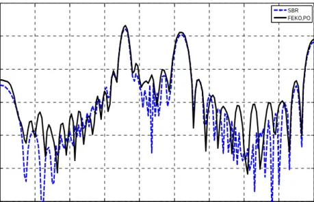
Figure 3.11 Comparison of PO and SBR results for θθ polarized monostatic RCS of PEC F-117 model ... 59 

Figure 3.12 Comparison of MoM and SBR results for θθ polarized monostatic RCS of PEC F-117 model ... 59 

1

CHAPTER 1

INTRODUCTION

During the second half of ₁₉th_{century, James Clerk Maxwell completed the} classical theory of electromagnetism, synthesizing all the previous knowledge developed by prominent physicists and mathematicians such as Coulomb, Ampere, Oersted, Faraday and Hertz. His famous equations, known as “Maxwell Equations”, have been widely used until the present time by physicists and engineers in numerous applications. A major application area of Maxwell’s equations is scattering of electromagnetic waves by obstacles. This topic gained a lot of importance after the development of radar systems during World War II. In radar applications, the electromagnetic power intercepted by a target is modeled via a hypothetical area known as Radar Cross Section (RCS). The power intercepted by the object is calculated as the product of RCS and the power density at the target location. As a result, calculation of the RCS of targets is one of the important aspects of radar engineering.

The RCS of an object is closely related of the constitutive parameters (permittivity, permeability and conductivity) and the geometry (or shape). In designing targets almost invisible to radars (i.e. stealth targets), it is the parameter that should be minimized. In early 1970s, stealth technology has become popular, with a lot of emphasis placed on reduction of the RCS of targets. Even though the modern view of stealth design is to achieve an optimum balance between RCS

2

reduction, incorporation of Electromagnetic Warfare (EW) and operational performance; RCS reduction is still the most important aspect of stealth technology. Modern radars are not only capable of detecting low RCS targets, but they can examine and classify targets according to their scattering characteristics. The main task of RCS design engineer is to introduce stealth targets effectively invisible to these powerful modern radars. At this point, developers of stealth targets use extensively the tools of Computational Electromagnetics (CEM) to simulate the scattering of electromagnetic waves by targets with complex geometry and/or electrical parameters.

The methods of CEM are based on the numerical approximation of Maxwell’s Equations for modeling the interaction of electromagnetic fields with objects. During the last few decades this area has become crucial for stealth engineering. The same methods are also used extensively in antenna design and placement, radome design, electromagnetic compatibility (EMC) analysis, RF component design and bio-electromagnetics problems. Many computational electromagnetics methods have been developed and implemented to solve different kinds of problems. Basically, these methods can be classified into two groups, namely as full-wave and approximate solution techniques.

Full-wave methods have been developed for the numerical discretization and approximation of equations deduced from Maxwell’s equations. The Method of Moments (MoM), Finite Difference Time Domain (FDTD) method and Finite Element Method (FEM) are the most commonly-used full-wave methods. These methods are sometimes named as low frequency methods because of the requirement of high computer resources at high frequencies. In recent years, some new full-wave based methods have been introduced in order to solve electrically large problems. For example, the Multilevel Fast Multi Pole Method (MLFMM) is a method that uses the formulation of MoM. Its main difference from the MoM is that it groups the basis functions and calculates the interaction between these groups. Through this modification, this approach can handle electrically large

3

problems such as dielectric structures with memory and run-time requirements formidable even for today’s super computers.

Approximate solutions are implemented basically to handle electrically large problems. Since these methods are effective at high frequencies, they are also known as high frequency solution techniques. Basic high frequency techniques are Physical Optics (PO), Geometric Optics (GO), Physical Theory of Diffraction (PTD), Geometric Theory of Diffraction (GTD) and Uniform Theory of Diffraction (UTD). PO and GO can give good solutions in specular regions but for complex structures their results are not very reliable. Utilization of GTD and PTD can improve the results of PO and GO in regions where diffracted rays dominate. In stealth designs, since specular reflections are avoided, calculation of the RCS must take into consideration the effect of diffraction and multiple reflections. Contribution of diffraction can be calculated with PTD. In recent years a new method, namely the Shooting and Bouncing Ray (SBR) method is implemented to solve the effects of multiple scattering. SBR is a method that uses a combination of the GO and PO techniques. It is a ray tracing technique suitable to use in stealth design applications.

1.1

Literature Review

Multiple Scattering plays an important role in RCS calculation. Cavity structures (such as jet-engine inlets) are the regions where multiple scattering phenomenon occurs. Since such structures contribute extensively to RCS, the analysis of this problem has been an important topic in RCS literature. Traditionally, RCS of cavity structures were calculated by model analysis or full wave methods. For complex structures, model analysis was not adequate, and full wave methods were not capable of solving electrically large problems. In 1987, SBR was implemented for the first time by Chou et al. [1] in a project work supported by NASA. In this method, rays are launched towards the cavity and traced inside with GO rules. Material properties of the cavity walls are taken into account and

4

rays are captured in the cavity opening in order to calculate the far field values. Later, Ling et al. presented this work as an article in [2].

SBR has been developed originally for cavity structures, but Baldauf et al. modified this technique for open scatterers [3]. In cavity structures, rays that leave the cavity are captured in the cavity opening. However for open scatterers the final integration aperture is not easy to choose. In [3], an aperture that coincides with the scatterer itself is suggested. With this aperture choice, the solution is identical to the conventional PO solution, except that multiple scattering effects of the rays are also modeled. In this work, formulation is based on Huygens’ Principle.

In 2005, to extend the capability of SBR for the simulation of scattering from diffusive and grating structures, Diffusive Ray Algorithm is introduced by Galloway et al. [4]. This algorithm reduces to the basic SBR formulation for targets constructed as a superposition of flat plates, but for curved structures a single ray tube that reflects from a curved part will generate a family of other ray tubes [4].

1.2

Overview of the Thesis

In this thesis, a basic SBR code is developed in MATLAB. Numerical results taken from the code are compared with the results obtained from FEKO software. FEKO is an electromagnetic (EM) analysis software which includes both full-wave and approximate solution methods and which has the capability to solve a wide range of electromagnetic problems [5]. For simple targets results are obtained from FEKO’s MoM and PO solvers. For electrically large problems results are obtained from MLFMM solver in a redhat based super computer with 18GB RAM.

5

SBR code is tested over simple targets like plate, dihedral and cube for monostatic and bistatic RCS calculations, for a range of frequencies. To test the SBR code for target in which multiple scattering phenomena is effective, a dihedral was used. Clearly, scattering from targets like dihedral and trihedral is dominated by multiple bounces and therefore composes a good test environment for SBR [3].

The code is implemented for open scatterers where the aperture chosen for final aperture integration becomes crucial. If the electromagnetic field values on the exit aperture were known exactly, regardless of the chosen exit aperture, exact far field result can be obtained [3]. Plane aperture and conformal aperture (coinciding with the scatterer itself) are implemented for final aperture integration. Results are critically evaluated to choose the best exit aperture to achieve accurate results.

Both for simple and complex targets, geometries are specified in STL mesh format. In STL mesh format, targets are constructed from triangular patches. Corner points and normal vectors of triangular patches are specified in this format. RCS is typically presented in plots of RCS values versus aspect angle. Aspect angle is the angle of target with respect to radar position. Different sweep configurations are implemented in the SBR code. For some cases, the target and receiver are fixed and the transmitter is rotated, for some cases the transmitter and receiver are fixed, and the target is rotated.

1.3

Outline of the Thesis

The thesis is organized in three main chapters. In Chapter 2 formulation of basic SBR algorithm is discussed. The code is tested over simple test targets like plate, cube, polyhedron and dihedral. Final aperture integration part of the code is discussed in detail and a new approach is developed in Chapter 2. Also, shadowing and multiple scattering are studied in this chapter.

6

In Chapter 3, application of SBR to complex targets is discussed. Methods of constructing a CAD model are studied. The chapter continues with the sweep definition. RCS of complex targets like ship, aircraft and tank are simulated in this part as well. Results are compared with FEKO results.

The thesis is summarized in Chapter 4. Advantages and disadvantages of the method are discussed. Concluding remarks are made on numerical results. The Chapter terminates with a summary of possible future work where possible modifications/enhancements of the algorithm are discussed.

7

CHAPTER 2

SHOOTING AND BOUNCING RAY METHOD

In this chapter, the Shooting and Bouncing Ray (SBR) method is discussed. It should be mentioned that the presented algorithm is a ray-based technique which can compute the RCS of electrically large, arbitrarily-shaped Perfect Electric Conductor (PEC) targets. Basically, the algorithm consists of ray tracing, amplitude tracking and final aperture integration parts.

The main blocks of the algorithm are discussed in Section 2.1. In Section 2.3, final aperture integration part of the algorithm is studied in details. Essentially, the algorithm is used to calculate the RCS of open scatterers. So, it is not convenient to perform the ray-tube integration over a common exit plane aperture [6]. SBR algorithm is powerful to calculate multiple scattering effects. In Section 2.4 this attribute of the algorithm is tested over problems dominated by multiple bounce effects. In Section 2.2 numerical results of SBR code are compared with the results of FEKO software. The last section is devoted to the shadowing effect.

8

2.1

Formulation of the Shooting and Bouncing Ray

Method

Shooting and Bouncing Rays (SBR) method is based on ray tracing. The problem is to determine the scattered field from an open scatterer. Basically, rays that simulate the incident plane wave are shot into the target, traced on the target and finally gathered in an exit aperture. Electric field is traced within the rays with Geometric Optic (GO) rules. The algorithm will be discussed in three main parts: 1) ray tracing 2) amplitude tracking and 3) physical optics approximation in exit aperture.

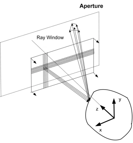
SBR uses both GO and PO rules. Referring to Figure 2.1 consider an arbitrary -shaped PEC object and an incident plane wave.

9

Figure 2.1 SBR, incident rays and exit aperture

The incident plane wave is represented by a dense grid of rays. A ray is defined by an origin,P =

(

x_p,y_p,z_p

)

and a direction vectorD=

(

s_x,s_y,s_z

)

. The equation for the ray is;

0 , ) (t = P+tD t ≥ I r (2.1) where,

10 i i x s =−sinθ cosφ (2.2) i i y s =−sinθ sinφ (2.3) i z s =−cosθ (2.4) i

θ and φi are angles that denote the direction of incidence.

The defined rays are shot into the PEC object. Let’s z= f(x,y) be the equation

of the surface of the scatterer. The intersection points of rays and the surface are found by solving equations of the surface and rays simultaneously. For example, if the object is a plate (i.e. the surface is a plane) we can find the intersection point as follows; a plane can be defined by a normal vector N and a point on the plane Q. A point P is on the plate if:

(

P−Q

)

=0

Nr (2.5)

By combining the equations of plane and ray together we end up with the following equation:

(

+ −

)

=0 × P tD Q Nr r (2.6) where D N P Q N t _{r r} r × − = ( ) (2.7)

For simple shapes like plate, sphere or cylinder a single implicit equation is enough to define the shape of the surface. For complex targets, a superposition of triangular patches can be used to approximate the geometry. In this case intersecting a ray with a triangle is more complicated than simple shapes. Basically, ray triangle intersection can be accomplished in two steps;

11

• Intersecting the ray and the plane of the triangle,

• Checking whether the intersection point is inside or outside the triangle.

Ray-plane intersection is already discussed in equations (2.5), (2.6) and (2.7). After finding the intersection point, we must decide whether the point is inside or outside the triangle. A triangle is defined with three vertices p0, p1 and p2. The normal vector of the triangle (n) is defined via the right hand rule.

p2-p0 p2 p1-p0 p1 p0 n

Figure 2.2 Triangle defined with right hand rule

) 0 2 ( ) 0 1 ( ˆ p p p p n= − × − (2.8)

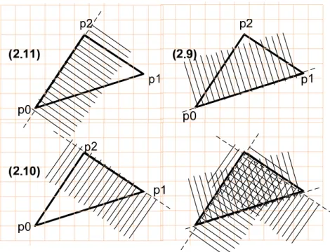
A triangle is the intersection of three half spaces as in Figure 2.3. Each edge of the triangle lies on a line and a point is inside the triangle if it is on the correct side of each one of the three lines [9].

12

Figure 2.3 A triangle constructed from three half spaces

Using this definition, a point is inside the triangle if it is on the left side of each edge. Via the cross product, it can be decided whether a point x is on the left or right of the edges with the following equations;

0 ˆ )) 0 ( ) 0 1 ((p − p × x− p ⋅n≥ (2.9) 0 ˆ )) 1 ( ) 1 2 ((p − p × x− p ⋅n≥ (2.10) 0 ˆ )) 2 ( ) 2 0 ((p − p × x− p ⋅n≥ (2.11)

Next, the reflected ray is determined by using the rules of Snell’s law [2]; 1) Reflected ray must lie in the plane of incidence

13

ˆ

i

ˆ

_i

N

ˆ

l z

ˆ

l x

ˆ

l y rayi rayr

ˆ

g x

ˆ

g y

ˆ

g z Global Coordinate System Local Coordinate System

Figure 2.4 Reflection of a ray

Referring to Figure 2.4 the reflected ray can be determined according to Snell’s law. A unit vector is defined as

i

i N

ray

mˆ =( × r)/sinθ (2.12)

where rayi is the incident ray and N is the reflection normal. Note that m is perpendicular to the plane of incidence. Referring to Figure 2.4, define the local coordinates m y_l = ˆ (2.13) N z_l =−r (2.14) ) ˆ (m N x_l =− × r (2.15)

14 ) , , (r θ φ ray_r = (2.16) 1 = r , θ =−(π/2−θˆ_i), φ =0 (2.17)

Next, (xl,yl,zl) coordinates of rayr in the local coordinate system can be

calculated by spherical to Cartesian coordinate transformation. As a final step local to global coordinate transformation is achieved as below;

⎥ ⎥ ⎥ ⎦ ⎤ ⎢ ⎢ ⎢ ⎣ ⎡ = 1 0 0 0 1 0 0 0 1 A (2.18) ⎥ ⎥ ⎥ ⎦ ⎤ ⎢ ⎢ ⎢ ⎣ ⎡ = ) 3 ( ) 2 ( ) 1 ( ) 3 ( ) 2 ( ) 1 ( ) 3 ( ) 2 ( ) 1 ( l l l l l l l l l z z z y y y x x x C (2.19) 1 − ⋅ = A C B (2.20) ) , , ( ) , , (xg yg zg =B⋅ xl yl zl (2.21)

where, Bis the transformation matrix. By using the reflected ray as a new incident ray this procedure is applied until the ray ends to bounce in the geometry.

In ray paths the field amplitude is also traced. In Geometrical Optics, the amplitude, phase and polarization of electric field can be updated with the following equation. φ j i i i i i i i i y z DF E x y z e x Er( ₊₁, ₊₁, ₊₁)=( ) .Γ.r( , , ). − (2.22) Where 2 1/2 1 2 1 2 1 0[(xi xi) (yi yi) (zi zi) ] k − + − + − = + + +

φ and DF_i is the divergence

factor which calculates the spreading of ray tubes. DF is applicable for curved surfaces and for planar surfaces takes the value of 1. Γi is the planar reflection

15

coefficient. For PECs, planar reflection coefficient can be applied with the equation (2.23). ) ˆ ) ˆ ( 2 ( ) ( E n E n Er = − i + × i × r r (2.23)

The scattered far field can be computed by applying the basic physical optics approximation in the aperture where exit rays are gathered. The magnetic current sheet Mr_s over the aperture is;

a

s E x y z n

Mr =2r( , , )× ˆ (2.24)

where, na

r _{is aperture normal.}

From this magnetic current sheet, the scattered field can be calculated. The scattered far field is the sum of contributions from individual ray tubes. The contribution of a ray tube is calculated as;

] ˆ ˆ [ 0 φ θ φ θ A A r e E i i r jk s = + − r (2.25) and, z E E Mr_s =[ _0θθˆ+ _0φφˆ]×2ˆ (2.26) where, z y x) ) ) ) _{θ φ θ φ θ}

φ =cos cos +cos sin −sin (2.27) y x) ) ) _{φ φ} θ =−sin +cos (2.28) ] ˆ ) sin( ) cos( ˆ ) cos( ) cos( [ 2 ] ˆ ) cos( ˆ ) [sin( 2E₀ y x E₀ y x Mr_s = _θ φ + φ + _φ − θ φ + θ φ (2.29)

16 dxdy e M jk A = 0

∫∫

_s jk.r 4π (2.30) ] sin cos [ 2 ) ( 0 0 i y i x uy ux jk E E dxdye jk A A φ φ π θ =

∫∫

_∑ + ⋅ + (2.31) ] cos ) cos sin [( 2 ) ( 0 0 i i y i x uy ux jk E E dxdye jk A A θ φ φ π φ =

∫∫

_∑ + ⋅ − + (2.32) i i u =sinθ cosφ (2.33) i i v=sinθ sinφ (2.34)

For the bistatic case, θi _and φi _{values in equations (2.31), (2.32), (2.33) and} (2.34) are replaced with observation angles.

Since the outgoing rays are not uniform, the integrations cannot be evaluated easily [2]. At this point, shooting and bouncing ray method has a way out. A small ray tube is shot into the geometry. The ray tube bounces on the geometry and comes to the aperture finally. Then the scattered field is calculated from this ray tube. Enough ray tubes are shot into the geometry to model the incident plane wave. The total scattered field is the sum of all contributions from the ray tubes.

ˆ

x

ˆ

y

ˆ

z Aperture Ray tube

17

Assume that the incident ray tube has an area of(Δx₀Δy₀). The central ray with

direction vector

(

sx,sy,sz

)

hits the aperture. The ray tube will have an area of

)

(ΔxsΔys on the aperture and the field within the existing ray tube can be approximated as )] ( ) ( [ 0 ) , ( ) , ( ) , ( ) , ( i y i x x x s y y s jk i i y i i x y x e y x E y x E y x E y x E _{− − + −} ⎥ ⎦ ⎤ ⎢ ⎣ ⎡ = ⎥ ⎦ ⎤ ⎢ ⎣ ⎡ (2.35)

This means that the amplitude of the field is same on the ray tube and across the ray tube there is a linear phase variation [2]. If the size of existing ray tube is too large, the approximation will not be valid. With equations below;

∑ ∫∫

+ − − + − = i tube ray y y s x x s jk vy ux jk x i y i e dxdye jk A 0 0( ) 0[ ( ) ( )] 2π θ ] sin ) , ( cos ) , ( [ i i i y i i i x x y E x y E φ + φ ⋅ (2.36)

∑ ∫∫

+ − − + − = i tube ray y y s x x s jk vy ux jk x i y i e dxdye jk A 0 0( ) 0[ ( ) ( )] 2π φ ] cos ) cos ) , ( sin ) , ( [( i i i i y i i i x x y E x y E φ + φ θ − ⋅ (2.37)

Since Ex(xi,yi) and Ey(xi,yi) are independent of integral variables they can be taken out of the integral;

∑

+ = i i i i y i i i x x y E x y E jk A [ ( )cos ( , )sin ] 2 0 _{φ φ} π θ i i i y s x s jk I y x e 0( x i y i)(Δ Δ ) ⋅ + (2.38)

∑

− + = i i i i i y i i i x x y E x y E jk

A [( ( )sin ( , )cos )cos ]

2

0 _{φ φ θ}

π

18 i i i y s x s jk I y x e 0( x i y i)(Δ Δ ) ⋅ + (2.39) where

∫∫

− + − Δ Δ = tube ray y s v x s u jk i i i y x dxdye y x I 0[( ) ( ) ] ) ( 1 (2.40)

The integral in equation (2.40) is the phase factor in standard physical optics theory [3]. Sometimes it is called shape function and it is the Fourier Transform of the ray tube shape.

In order to take advantage of this method for each ray tube, four rays around a central ray are shot into the geometry.

Figure 2.6 Shape of exit ray tube

The position vectors of rays are denoted byγrnˆ =xnxˆ+ynyˆ, n=1,2,3,4. Fourier transform can be evaluated as described in [2], [7]. Simpler proof of this method based on Stokes’ theorem can also be considered in [10].

19 ) 0 , 0 ( / ) , (p q S S Ii = (2.41) where,

∑

= − − + + − + − + • − + − − + − − − − − − = 4 1 1 1 1 1 1 1 1 1 ] ) ( ) ][( ) ( ) [( ) )( ( ) )( ( ) , ( n n n n n n n n n n n n n n n n n jw q y y p x x q y y p x x x x y y y y x x e q p S γn (2.42) 2 / ) ( ) ( ) ( ) ( ) 0 , 0 ( x₁y₂ x₂y₁ x₂y₃ x₃y₂ x₃y₄ x₄y₃ x₄y₁ x₁y₄ S = − + − + − + − (2.43) ) ( 0 u sx k p= − (2.44) ) ( 0 v sy k q= − (2.45) y q x p wr = ˆ+ ˆ (2.46)

As a final step, RCS can be calculated as in equations (2.47) and (2.48).

2 4π Aθ RCS = ⋅ (Vertical polarization) (2.47) 2 4π A_φ RCS = ⋅ (Horizontal polarization) (2.48)

2.2

Numerical Results for Simple Targets

In this section, RCS values of some simple targets are compared with Method of Moments (MoM) and Physical Optics (PO) results. FEKO, a software product for the simulation of electromagnetic fields, is used to obtain MoM and PO results. Different solution techniques implemented within FEKO make it applicable for a wide range of problems [5]. The targets of interest are a plate, a cube and a flare- like shape. Generally, monostatic RCS of targets were calculated for vertical polarization. Targets are swept in

θ

angle. FEKO software runs on computers; Computer 1; Intel (R) Core 2 Duo CPU, [email protected]

3.25GB RAM

Computer 2; (Dual) AMD Opteron ™ Processor 248 14.926 GB RAM

20

Computer 2 is used for electrically large problems. Even with computer 2 some problems cannot be solved with MoM. Multilevel Fast Multipole Method (MLFMM) which is a fast alternative formulation of the MoM is applicable to much larger structures than the MoM [5]. MLFMM makes it possible to obtain full-wave solutions for electrically large structures [5]. With this method and computer 2, a military aircraft at 2.5GHz or a ship at 400MHz can be handled. In order to solve the same problems with MoM, we need 30TByte memory approximately.

Different sweep geometries are used to calculate the RCS values of simple PEC obstacles. In the plate geometry, plane wave (provided by the transmitter) is swept around the target in θ angle and plate is kept fixed in origin. For cube and flare like shape, transmitter and exit aperture (in the direction of the receiver) are kept fixed and the target is rotated in y axis. Both approaches can be used to calculate the monostatic RCS.

The plate geometry is formulated in the problem directly by using its equation. The cube and flare like geometry are created from triangle patches that are big enough to permit to construct these shapes. The number of the triangular patches is kept minimal to decrease the runtime since the SBR code generated in MATLAB does not include a special algorithm that speeds up the ray-triangle intersection test. Ray-triangle intersection is tested with brute force methods, which implies that runtime increases dramatically with the number of patches.

The first simulation was conducted on a perfect electric conductor (PEC) flat plate as illustrated in Figure 2.7. In this simulation both monostatic and bistatic RCS of a square PEC plate with side length of 0.25 meters were computed and compared with MoM and PO results taken from FEKO.

21

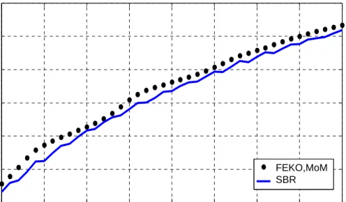
The plate was illuminated from φ ₌₀o _and θ ₌₀o_{and its monostatic RCS was} computed with respect to frequency from 2GHz to 6GHz as shown in Figure 2.7. The result of the SBR is compared with the MoM and given in Figure 2.8.

Figure 2.7 Simulation setup for monostatic RCS of PEC plate

Rays are shot towards the plate with λ/10 density, where λ is wave length. For each ray, four rays neighboring the central ray are shot to build up a ray tube. Since specular reflections are dominant, the results of SBR solution and MoM are perfectly matched.

22 2 2.5 3 3.5 4 4.5 5 5.5 6 2 4 6 8 10 12 14

Monostatic RCS of a PEC plate with respect to frequency

frequency [GHz] RC S [ d Bm 2 ] MOM Standard SBR FEKO,MoM SBR

Figure 2.8 Comparison of MoM and SBR results for θθ polarized monostatic RCS of PEC

plate with respect to frequency

For bistatic case, the plate is illuminated from φ ₌₀o _and θ ₌₋₁₀o_{and its bistatic} RCS is computed at φ ₌₀o _and θ ₌₁₀o _{with respect to frequency from 2GHz to} 6GHz as shown in Figure 2.9. The result of the SBR was compared with the MoM and given in Figure 2.10.

23

Figure 2.9 Simulation setup for bistatic RCS of PEC plate

As a result for flat surfaces in specular regions the results are matching with MoM results perfectly for both monostatic and bistatic cases.

2 2.5 3 3.5 4 4.5 5 5.5 6 2 4 6 8 10 12 14 frequency [GHz] RCS [ d B m 2 ]

Bistatic RCS of a PEC plate with respect to frequency

MOM

Standard SBR

FEKO,MoM SBR

Figure 2.10 Comparison of MoM and SBR results for θθ polarized bistatic RCS of PEC

24

In the following example, the plate is illuminated at _{φ =0}o _{from θ =−60}o_to o

60

=

θ and its monostatic RCS is computed Figure 2.11. The result of the SBR was compared with the MoM in Figure 2.12 and with PO in Figure 2.13.

25 -60 -40 -20 0 20 40 60 -30 -25 -20 -15 -10 -5 0 5 10 15

Monostatic RCS of PEC Plate

Theta [degrees] RC S [ d Bm 2] SBR FEKO, MoM

Figure 2.12 Comparison of MoM and SBR results for θθ polarized monostatic RCS of PEC

plate

The results are perfectly matching with MoM near specular region. Results are not agreeing at angles where diffraction effects are dominant. SBR code is unable to model diffraction. When we compare the results with PO code in FEKO we can see that the results are in good agreement, since PO is also unable to take diffraction into account.

26 -60 -40 -20 0 20 40 60 -50 -40 -30 -20 -10 0 10 20 Theta [degrees] RCS [ d B m 2]

Monostatic RCS of PEC plate

FEKO, PO SBR

Figure 2.13 Comparison of PO and SBR results for θθ polarized monostatic RCS of PEC

plate

In the other case the plate is illuminated from φ ₌₀o _and θ ₌₀o_{and its bistatic} RCS is computed at φ ₌₀o _from θ ₌₋₉₀o_to θ ₌₉₀o _{as in Figure 2.14. The result} of the SBR was compared with the MoM and given in Figure 2.15.

27

Figure 2.14 Simulation setup for bistatic RCS of PEC plate

The results are harmonious with MoM near specular regions. In rear sides where diffraction contribution is important, the results are not matching well with the MoM results.

28 2 2.5 3 3.5 4 4.5 5 5.5 6 -40 -35 -30 -25 -20 -15 -10 -5 0 5 frequency[GHz] RC S[ d B m 2]

Bistatic RCS of PEC plate

SBR FEKO,MoM

Figure 2.15 Comparison of MoM and SBR results for θθ polarized bistatic RCS of PEC

plate

Finally, for the plate case, bistatic RCS is computed with respect to frequency. The plate is illuminated from φ ₌₀o _andθ ₌₀o_{, RCS values are computed at}

o 0

=

φ and θ ₌₁₅o _{with respect to frequency from 2GHz to 6GHz as shown in} Figure 2.16. The result of the SBR was compared with the MoM and given in Figure 2.17.

29

Figure 2.16 Simulation setup for bistatic RCS of PEC plate

Out of the specular region where diffraction mechanism is effective, again the results are not in agreement with MoM results. Hence, it can be concluded that by correctly modeling the diffraction effects, more accurate results can be obtained out of specular regions.

30 2 2.5 3 3.5 4 4.5 5 5.5 6 -40 -35 -30 -25 -20 -15 -10 -5 0 5 frequency [GHz] RCS [ d B m 2]

Bistatic RCS of PEC plate

SBR FEKO, MoM

Figure 2.17 Comparison of MoM and SBR results for θθ polarized bistatic RCS of PEC

plate with respect to frequency

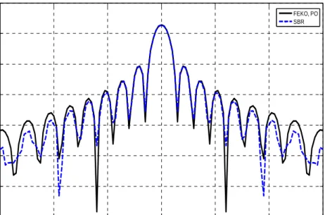
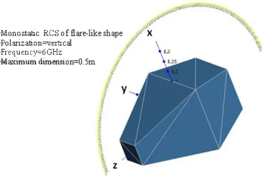
The second example was conducted on a flare like object shown in Figure 2.18. The object is represented by 20 triangle patches. Maximum length of the object is 0.5 meter. The monostatic RCS is calculated at _{φ =0}o _from θ ₌₀o_to θ ₌₁₈₀o _for vertical polarization at 6GHz. For each monostatic RCS value 72000 rays are traced with λ/10 density. Results are compared with the PO solution in Figure 2.19.

31

Figure 2.18 Simulation setup for monostatic RCS of PEC flare-like shape

For the angle ranges ₁₅0 _{<θ <50}0_{, 80}0 _{<θ <90}0 _{and 120}0 _{<θ <160}0_{, the RCS} values are not matching with PO results. This discrepancy between the results is due to the shape of the aperture over which the rays are collected. At these angles, some of the rays bouncing from the geometry cannot be gathered at the planar exit aperture. After a detailed analysis, it is seen that the aperture shape must be modified in order to obtain correct results. Alternative solution suggestions and formulations related to this point are considered in Section 2.3. In this section, it will be shown that conformal apertures that encompass the scatterer are effective in collecting rays in a proper fashion. Although this point will be fully clarified in the next section, corrected results obtained by a conformal aperture are represented in Figure 2.20. With this new formulation that will be presented in Section 2.3, results agree very well with the PO solution.

32 0 20 40 60 80 100 120 140 160 180 -40 -30 -20 -10 0 10 20

Monostatic RCS of PEC flare-like shape

Theta [degrees] RCS [ d B m 2] SBR FEKO,PO

Figure 2.19 Comparison of PO and SBR results for θθ polarized monostatic RCS of PEC

flare-like shape for planar aperture case

Results in Figure 2.20 show that SBR algorithm gives the same results as PO solution. Additionally, ray tracing capability of the code handles the multiple scattering and shadowing problems.

33 0 20 40 60 80 100 120 140 160 180 -40 -30 -20 -10 0 10 20

Monostatic RCS of PEC flare-like shape

Theta [degrees] RCS [ d B m 2] SBR FEKO,PO

Figure 2.20 Comparison of PO and SBR results for θθ polarized monostatic RCS of PEC

flare-like shape for conformal aperture case

The third example was conducted on an arbitrary prism shown in Figure 2.21. The shape is composed of 14 triangular patches. The maximum length of the shape is 0.35 meters. Monostatic RCS is calculated at φ ₌₀o _from θ ₌₀o_to θ ₌₃₆₀o _for vertical polarizations at 5GHz. The results are compared with PO and MoM results.

34

Figure 2.21 Simulation setup for monostatic RCS of PEC arbitrary polyhedron

0 50 100 150 200 250 300 350 -40 -30 -20 -10 0 10 20

Monostatic RCS of arbitrary polyhedron

Theta [degrees] R C S [ d Bm 2] FEKO,PO SBR

Figure 2.22 Comparison of PO and SBR results for θθ polarized monostatic RCS of PEC

35

In Figure 2.22, it is seen that the results are close to the PO solution except for angles from θ ₌₆₀o _{up to}θ ₌₁₃₀o_{. The problem at these angles can be revealed} when the geometry is investigated more closely in Figure 2.24. At problematic aspect angles, rays that are shot towards the geometry are intersecting with four points located on the surface. The naive ray tracing algorithm of the code is unable to handle such situations, where the object is concave and a ray may intersect with several points on the surface. In section 2.5, it is explained how the algorithm is overviewed to overcome this problem. SBR is a ray tracing method and naturally ray tracing algorithms may correctly handle the shadowing problem. Although the modifications introduced in the code are explained in Section 2.5, the correct results obtained after these amendments are shown in Figure 2.23.

0 50 100 150 200 250 300 350 -40 -30 -20 -10 0 10 20

Monostatic RCS of arbitrary polyhedron

Theta [degrees] RC S [ dBm 2] SBR FEKO,PO

Figure 2.23 Comparison of PO and SBR results for θθ polarized monostatic RCS of PEC

arbitrary polyhedron after correction on shadowing algorithm

After these modifications on the code, the results agreed with the PO solution except at angles₁₉₀0 _{<θ <230}o_{. At these angles, multiple scattering is dominant.}

36

For this example, multiple scattering is not implemented in the code. The results are also compared with the MoM results. In Figure 2.25, multiple scattering effects can be seen in MoM results in an obvious fashion. Multiple scattering effects will be implemented in Section 2.4.

37 0 50 100 150 200 250 300 350 -40 -30 -20 -10 0 10 20 Theta [degrees] RC S [ d Bm 2]

Monostatic RCS of arbitrary polyhedron

FEKO,MoM FEKO,PO SBR

Figure 2.25 Comparison of PO, MoM and SBR results for θθ polarized monostatic RCS of

PEC arbitrary polyhedron

The fourth example was conducted on an arbitrary polyhedron shown in Figure 2.26. The shape is composed of 8 triangular patches. The maximum length of the shape is 0.3 meters. The monostatic RCS is calculated at _φ=0o _{from θ =0}o_to

o 180

=

θ for vertical polarizations at 5GHz. The results are compared with PO and MoM results.

38

Figure 2.26 Simulation setup for monostatic RCS of PEC arbitrary polyhedron

0 20 40 60 80 100 120 140 160 180 -60 -50 -40 -30 -20 -10 0 10

Monostatic RCS of arbirary shape

Theta [degrees] RCS [ d B m 2] SBR FEKO,PO

Figure 2.27 Comparison of PO and SBR results for θθ polarized monostatic RCS of PEC

39

The results agree very well with the PO solution for this arbitrary polyhedron. The main reason for this conclusion is the convex shape of the object that avoids all the difficulties encountered in the previous example.

2.3

SBR Final Integration Aperture

The Shooting and Bouncing Ray method has been first applied on cavity structures like a jet inlet or an aircraft cabin [2], where open mouth of the cavity has been chosen as the final integration aperture. However, for open scatterers there are several options for the choice of an aperture choose. If the exit aperture is chosen as planar, this choice gives good results in specular regions. A planar aperture cannot be adequate for gathering the exit rays for some problems. Basically, the problem can be investigated by using the cube geometry shown in Figure 2.28. With a planar exit aperture, it is not possible to collect outgoing rays at angles close to 45 degrees. By fixing the transmitter (plane wave) and exit aperture (receiver) and rotating the geometry, the monostatic RCS of the cube can be calculated as shown in Figure 2.29.

40

Figure 2.28 Planar exit aperture approach

At angles₀0 _{<θ <30}0_{, 60}0 _{<θ <120}0 _{and 150}0 _{<θ <180}0 _{the results are in} good agreement with both MoM and PO results. On the other hand, at angles between ₃₀0 _{<θ <60}0 _{and 120}0 _{<θ <150}0 _{the field values are well below those} obtained by MoM and PO. At 45º SBR code yields −∞ value. If the MoM and PO results are evaluated together, the difference between them in these problematic angles is not much. So, it can be stated that the problem is not due to the absence of diffraction effect in the code. At angles near 45º the rays bouncing from cube cannot be gathered at the planar aperture. This leads us to state that contribution of rays at these angles are greater than diffraction effects, and their contribution to the RCS value must be taken into account. To overcome this problem, a new exit aperture is recommended and formulated.

41 0 20 40 60 80 100 120 140 160 180 -50 -40 -30 -20 -10 0 10 Thetas [degrees] R C S [ d Bm 2]

Monostatic RCS of PEC cube

SBR,Planar Aperture FEKO,MOM FEKO,PO

Figure 2.29 Monostatic RCS of PEC cube with planar exit aperture approach

A conformal exit aperture as shown in Figure 2.30 can be the best choice to gather the exit rays. In conformal exit aperture, all outgoing rays are gathered and their contributions to overall RCS value can be calculated. Basically, the conformal exit aperture is a replica of the geometry of the surface itself. This guaranties that all rays bouncing from the geometry can be evaluated for their contribution to RCS.

Formulation of a conformal exit aperture is more complicated than a planar exit aperture formulation [8]. In order to simplify the resulting equations, for each element (planar part) of the conformal exit aperture, a local coordinate system

) , ,

(xl yl zl shall be defined as shown in Figure 2.30. The local coordinates are defined using the following equations;

N

42

N is the normal of the triangular patch with which the rays intersect. To define a local coordinate system, local z coordinate is projected into global x, y plane according to the following equation;

z z l l z a a z u= −( ⋅ )) (2.50)

Then, to find the global-to-local transformation matrix, rotation angles φ and θ are calculated by means of equations (2.51) and (2.52).

) / ] ( cos 1 u u a_x ⋅ = − φ (2.51) ) / ] ( cos 1 N N a_z ⋅ = − θ (2.52)

The global-to-local transformation matrix can be defined through the multiplication of rotation matrices.

⎥ ⎥ ⎥ ⎦ ⎤ ⎢ ⎢ ⎢ ⎣ ⎡ − × ⎥ ⎥ ⎥ ⎦ ⎤ ⎢ ⎢ ⎢ ⎣ ⎡ − = ) cos( 0 ) sin( 0 1 0 ) sin( 0 ) cos( 1 0 0 0 ) cos( ) sin( 0 ) sin( ) cos( θ θ θ θ φ φ φ φ T (2.53)

After defining the local coordinate system values in equation (2.42) and (2.43), are transformed into local coordinate system. Then, the incident field given in the global coordinate system is transformed into the local coordinate system as follows: T z y x E z y x E g g g i l l l i_{( , , )}= _{( , , )}⋅ _(2.54)

Finally, φ and θ parameters in equation (2.51) and (2.52) are used in equations (2.31) and (2.32).

43 l x l y zl l z l x l y l x l y l z l z l x l y z y

x

Figure 2.30 Conformal exit aperture approach

With aperture modification, at angles between ₃₀0 _{<θ <60}o_{and 120}0 _{<θ <150}o the calculated values agree well with MoM and PO results as shown in Figure 2.31.

44 0 20 40 60 80 100 120 140 160 180 -50 -40 -30 -20 -10 0 10 Theta [degrees] R C S [ d Bm 2]

Monostatic RCS of PEC cube

SBR, Conformal Aperture FEKO,PO FEKO,MoM

Figure 2.31 Monostatic RCS results with conformal exit aperture approach

2.4

SBR Multiple Scattering Capability

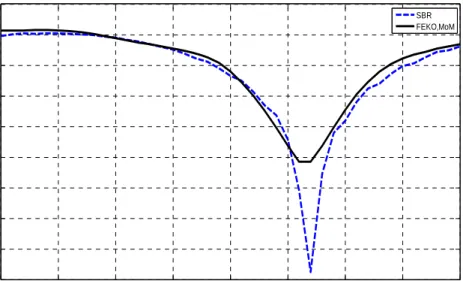
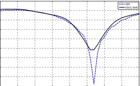
In the SBR code, rays must be allowed to bounce within the geometry until they exit. The structure of the algorithm allows us to compute multiple scattering effects without a limit unless we have extremely long runtimes. With non-convex targets that have concave surfaces such as cavities and corners, numerical results of PO deviate from our simulation results. Targets like dihedral and trihedral are appropriate to test the code for multiple scattering capabilities.

A PEC dihedral shown in Figure 2.32 will be a good test object for SBR code. Clearly, scattering from a dihedral is dominated with multiple scattering effects. As shown in Figure 2.32 a dihedral is illuminated from θ ₌₋₆₀o _to θ ₌₆₀o_and its monostatic RCS was computed with respect to θ at 6GHz.

45

Figure 2.32 Simulation setup for monostatic RCS of PEC dihedral

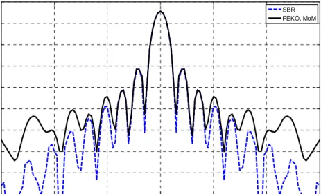
In Figure 2.33 results are obtained with and without considering the multiple scattering effects. Clearly, the RCS values for a problem where multiple scattering is dominant are not matching with MoM results when multiple scattering is not modeled in the code.

The SBR RCS values are in good agreement with the MoM results when multiple scattering mechanism is implemented in the code.

46 -60 -40 -20 0 20 40 60 -50 -40 -30 -20 -10 0 10 Theta [degrees] R C S [ d Bm 2]

Monostatc RCS of PEC dihedral

SBR FEKO, MoM FEKO, PO

SBR, w/o multiple scattering capability

Figure 2.33 Comparison of PO, MoM and SBR results for θθ polarized monostatic RCS of

PEC dihedral

2.5

Shadowing

For a specific aspect angle, the incident electromagnetic wave illuminates some parts of the target and the rest of the target will stay in dark. In addition, some parts of the target can be shadowed by other parts of the target itself. Especially, concave and separated parts of targets cause shadowing. For example, wings of airplanes induce shadowing from certain aspect angles over the body of the aircrafts. Many algorithms are developed to solve this problem for the PO approach.

Naturally, SBR is using the ray tracing method, which handles the shadowing effect in a natural way. Basically, if a ray intersects with a part of the target for

47

the first time, this part will be the illuminated part and the rest will stay in the shadow region.

Figure 2.34 Shadowing problem

In Figure 2.34, triangle 9 is shadowed by triangle 15. The ray intersects first triangle 15 which is taken as the illuminated part. As a summary, ray tracing is itself a natural shadowing algorithm. Ray tracing is implemented to find the ray-triangle intersection points, and the primary intersection part is taken as the illuminated part, and the rest are assumed to lie in shadow.

48

CHAPTER 3

APPLICATION OF SBR TO COMPLEX TARGETS

In the previous chapter, the SBR code is tested by using simple PEC objects. However, realistic targets possess much more complex geometries with several scattering mechanisms. The interactions between parts of complex geometries will affect dramatically the RCS values. At this point the SBR code, with its multiple scattering capability, will be superior to other ray based RCS prediction tools. The RCS prediction code developed in the previous chapter will be applied to complex targets in this chapter, in order to evaluate the performance of the method for realistic cases.

In our simulations, targets are modeled using large triangular patches. In order to calculate the monostatic RCS of a target from different aspect angles, two different methods are used. In the first method, the target kept fixed and the ray window in Figure 3.1 is rotated. This method is applied to simple shapes.

49

Figure 3.1 Target and Ray Window Geometry

In the second method, which is used for complex targets, the target is rotated.

3.1

Target Modeling

By using a superposition of simple primitive objects like prisms, spheres or cylinders, complex targets can be modeled. However, such models may suffer from precision. Surface patch representations will yield accurate target models. Triangular patches are very flexible for modeling targets effectively. However, if our geometric model has a large number of patches, the ray-triangle intersection algorithm will be the main contributor to runtime. By using brute force search techniques it is not possible to solve high frequency problems in reasonable times. In our examples, we construct geometries by using large triangular patches shown in Figure 3.3. The geometries are constructed in a Computer Aided Design (CAD)

50

modeling tool. The geometry is imported in STL mesh format shown in Figure 3.2 and used in SBR MATLAB code.

Figure 3.2 STL mesh structure

Although complex targets are considered in this section, we start with a simple case to remember the essential points in RCS calculations. For a single triangular patch shown in Figure 3.3, the monostatic RCS value is calculated. In the specular region SBR results agree very well with MoM results. Outside the specular region, where diffraction is effective, SBR results are deviating from MoM results. Since our complex targets are all composed of triangular patches, it can be claimed that those patches contributing to specular reflection will dominate. In the absence of such patches, SBR and MoM will not match, due to the dominant diffraction effects. In the following examples, three different complex targets are

51

simulated; first a tank model which is modeled by 132 triangular patches, second a simple ship model constructed from 28 triangular patches and last a stealth aircraft design constructed from 20 triangular patches, which is more like an F-117 aircraft.

Figure 3.3 Simulation setup for monostatic RCS of PEC triangular patch

-60 -40 -20 0 20 40 60 -40 -35 -30 -25 -20 -15 -10 -5 0 5 10 15 Theta[degrees] RC S [d B m 2]

Monostatic RCS of PEC triangle

SBR FEKO,MoM

Figure 3.4 Comparison of MoM and SBR results for θθ polarized monostatic RCS of PEC

52

3.2

Target Rotation

For the visualization of RCS variation, we obtain plots of RCS versus aspect angles. Aspect angle is the orientation of target relative to the source position which is a ray window. In order to calculate the RCS as a function of aspect angle, the target is rotated. In order to rotate the target in three dimensions, three basic rotation matrices are used;

⎥ ⎥ ⎥ ⎦ ⎤ ⎢ ⎢ ⎢ ⎣ ⎡ − = ) cos( ) sin( 0 ) sin( ) cos( 0 0 0 1 ) ( α α α α α x R (3.1) ⎥ ⎥ ⎥ ⎦ ⎤ ⎢ ⎢ ⎢ ⎣ ⎡ − = ) cos( 0 ) sin( 0 1 0 ) sin( 0 ) cos( ) ( α α α α α y R (3.2) ⎥ ⎥ ⎥ ⎦ ⎤ ⎢ ⎢ ⎢ ⎣ ⎡ − = 1 0 0 0 ) cos( ) sin( 0 ) sin( ) cos( ) ( α α α α α z R (3.3)

Each of these matrices rotates a target in counterclockwise direction around a fixed coordinate axis, by an angle ofα . Rotation direction is determined by the right-hand rules. Other rotation matrices are derived from these three basic matrices.

In our simulations, for rotating a target that is in STL mesh format, all vertices of triangular patches are rotated about the orthogonal axes of the global coordinate system. Simple rotation geometry is illustrated in Figure 3.5.

53

Figure 3.5 Fixed rotation around Y axis

3.3

Numerical Results

The first simulation is conducted on a simple tank model which has a length of 1 m and a height of 0.5 m. Monostatic RCS values are calculated at angles from

o 0

=

θ to _{θ =180}o _{at 6GHz. The results obtained from SBR MATLAB code are} compared with those obtained from the FEKO software. In these simulations, two computers are used;

Computer 1; Intel (R) Core 2 Duo CPU, [email protected] 3.25GB RAM

Computer 2; (Dual) AMD Opteron ™ Processor 248 14.926 GB RAM

The tank is modeled in CADFEKO, which is the modeling tool of FEKO software, and exported in STL mesh format. The model consists of 132 triangular patches.

54

Figure 3.6 Tank model constructed from 132 triangular patches

Table 3-1 Computation times for tank model simulation

Time/Sample Seconds Sample Total Time Hours RAM MB Computer SBR, MATLAB 1181 181 59.4 --- 1 PO, FEKO 0.19 181 0.01 13 1

55 -80 -60 -40 -20 0 20 40 60 80 -60 -50 -40 -30 -20 -10 0 10 20 Theta [degrees] RC S[ d B m 2]

Monostatic RCS of tank model

FEKO,PO SBR

Figure 3.7 Comparison of PO and SBR results for θθ polarized monostatic RCS of PEC

tank model

The results of FEKO (PO) and MATLAB (SBR) match closely as shown in Figure 3.7. Although the model contains only a moderate number of patches, the runtime is very long due to the lack of a fast ray-triangle intersection algorithm. With brute-force ray-triangle intersection test, it takes 20 minutes to calculate the monostatic for a single aspect angle.

The second example is conducted on a simple ship model with length 1 m and height 0.5 m. Monostatic RCS values are calculated at angles from θ ₌₀o _to

o 180

=

θ at 6GHz. The ship is modeled in CADFEKO, modeling tool of FEKO software, and exported in STL mesh format. The model consists of 28 triangular patches. In this example, the solution is obtained by using a planar exit aperture. Although we have mentioned that the conformal aperture approach yields optimum results, this example shows that the planar exit aperture choice can give good results for targets whose scattering characteristics are dominated with specular regions.

56

Figure 3.8 Monostatic RCS of ship model

Table 3-2 Computation times for ship model simulation

Time/Sample Seconds Sample Total Time Hours RAM MB Computer SBR, Matlab 551 151 23.2 --- 1 PO, FEKO 0.25 181 0.012 13 1 MLFMM, FEKO 2880 31 24.9 875 2

57 0 20 40 60 80 100 120 140 160 180 -30 -25 -20 -15 -10 -5 0 5 10 15 20 25 Theta [degrees] R C S [ d Bm 2]

Monostatic RCS of ship model

SBR FEKO, PO FEKO, MLFMM

Figure 3.9 Comparison of PO, MLFMM and SBR results for θθ polarized monostatic RCS

of PEC ship model

The results obtained from FEKO (PO and MLFMM) and SBR agree well in specular regions. Due to the fact that specular scattering is dominant in this model the results match closely with those obtained by FEKO (MLFMM) in the wide spectrum from _{θ =0}o _{toθ =180}o