Frequency-dependent functional connectivity within resting-state networks: An atlas-based MEG beamformer solution

(1)

Frequency-dependent functional connectivity within resting-state networks: An

atlas-based MEG beamformer solution

Arjan Hillebrand

a,

⁎

, Gareth R. Barnes

b

, Johannes L. Bosboom

c

, Henk W. Berendse

d

, Cornelis J. Stam

a

Department of Clinical Neurophysiology and Magnetoencephalography Center, VU University Medical Center, Amsterdam, The Netherlands b_{Wellcome Trust Centre for Neuroimaging, University College London, London WC1N 3BG, UK}

c

Onze Lieve Vrouwe Gasthuis, Amsterdam, The Netherlands d

Department of Neurology, VU University Medical Center, Amsterdam, The Netherlands

a b s t r a c t

a r t i c l e i n f o

Article history: Received 20 July 2011 Revised 27 October 2011 Accepted 2 November 2011 Available online 9 November 2011 Keywords: Beamforming Magnetoencephalography Source modelling Functional connectivity Graph analysis Networks Phase lag index Resting-state

The brain consists of functional units with more-or-less speciﬁc information processing capabilities, yet cog-nitive functions require the co-ordinated activity of these spatially separated units. Magnetoencephalography (MEG) has the temporal resolution to capture these frequency-dependent interactions, although, due to vol-ume conduction andﬁeld spread, spurious estimates may be obtained when functional connectivity is esti-mated on the basis of the extra-cranial recordings directly. Connectivity estimates on the basis of reconstructed sources may similarly be affected by biases introduced by the source reconstruction approach. Here we propose an analysis framework to reliably determine functional connectivity that is based around two main ideas: (i) functional connectivity is computed for a set of atlas-based ROIs in anatomical space that covers almost the entire brain, aiding the interpretation of MEG functional connectivity/network studies, as well as the comparison with other modalities; (ii) volume conduction and similar bias effects are removed by using a functional connectivity estimator that is insensitive to these effects, namely the Phase Lag Index (PLI).

Our analysis approach was applied to eyes-closed resting-state MEG data for thirteen healthy participants. Wefirst demonstrate that functional connectivity estimates based on phase coherence, even at the source-level, are biased due to the effects of volume conduction andfield spread. In contrast, functional connectivity estimates based on PLI are not affected by these biases. We then looked at mean PLI, or weighted degree, over areas and subjects and found significant mean connectivity in three (alpha, beta, gamma) of thefive (includ-ing theta and delta) classical frequency bands tested. These frequency-band dependent patterns of rest(includ-ing- resting-state functional connectivity were distinctive; with the alpha and beta band connectivity confined to poste-rior and sensorimotor areas respectively, and with a generally more dispersed pattern for the gamma band. Generally, these patterns corresponded closely to patterns of relative source power, suggesting that the most active brain regions are also the ones that are most-densely connected.

Our results reveal for theﬁrst time, using an analysis framework that enables the reliable characterisation of resting-state dynamics in the human brain, how resting-state networks of functionally connected regions vary in a frequency-dependent manner across the cortex.

Introduction

The brain consists of billions of interconnected neurons, forming an extremely complex system (Tononi and Edelman, 1998; Tononi et al., 1998) in which clusters of neurons are organised as functional units with more-or-less speciﬁc information processing capabilities (e.g.

Born and Bradley, 2005; Grodzinsky, 2000). Yet, cognitive functions re-quire the coordinated activity of these spatially separated units, where

the oscillatory nature of neuronal activity, and phase relations between units, may provide a possible mechanism (Fries, 2005; Varela et al., 2001). Not only has it been shown that rhythmic activity plays an im-portant role in perception and sensori-motor systems (Arieli et al., 1996; Forss and Silen, 2001; Hari and Salmelin, 1997; Houweling et al., 2010; Kenet et al., 2003; Linkenkaer-Hansen et al., 2004; Mima et al., 2000), as well as in higher cognitive functions (Engel et al., 2001; Ward, 2003), but it has also been shown that patterns of resting-state oscillatory activity in patients with neurological disorders differ from those in healthy subjects, and that these differences correlate with cog-nitive performance (Uhlhaas and Singer, 2006).

Magnetoencephalography (MEG), with its high temporal resolu-tion, can be used to characterise the (resting-state) networks formed ⁎Corresponding author. Fax: +31 020 4444816.

doi:10.1016/j.neuroimage.2011.11.005

Contents lists available atSciVerse ScienceDirect

NeuroImage

j o u r n a l h o m e p a g e : w w w . e l s e v i e r . c o m / l o c a t e / y n i m g

Open access under CC BY license.

(2)

by interacting sources of oscillatory activity (Bassett et al., 2006; Hyvarinen et al., 2010; Langheim et al., 2006; Liu et al., 2010). However, in many MEG studies the required estimation of functional connectiv-ity is performed at the sensor-level, which impedes comparison with the rapidly growing literature on resting-state functional connectivity using functional Magnetic Resonance Imaging (fMRI;van den Heuvel and Hulshoff Pol, 2010). Another problem is that multiple recording sites pick up signals from a single source due to both the nature of the induced magneticﬂux (see e.g.Domínguez et al., 2007) and volume conduction, which can lead to erroneous estimates of functional con-nectivity when these estimates are based on sensor-level measure-ments. Moreover, the signals originating from spatially separated brain areas are mixed at the sensor level, which can result in over/un-derestimation of synchronisation, where the exact effect is dependent on a complex interplay of modulations in source- and noise-power, source interactions, as well as relative position and orientation of the sources (e.g.Grasman et al., 2004; Meinecke et al., 2005; Schoffelen and Gross, 2009).

These limitations have provoked research into four different direc-tions: i) using estimates of the expected functional connectivity that is due to volume conduction/field spread without true interactions, and subtracting such estimates from the measured functional connectivity (Nunez et al., 1997), or using such estimates to derive a statistical threshold for the measured interactions (e.g.Brookes et al., 2011a); ii) the development of functional connectivity estimators that are in-sensitive to these confounds offield spread and volume conduction (Nolte et al., 2004; Stam et al., 2007); iii) development of techniques such as DCM (Dynamic Causal Modelling;Friston et al., 2011; Moran et al., 2009) that, given a set of hypotheses, test between different bio-physically motivated source- or network-models based on their model evidence; and iv) investigations into the utility of functional connectivity analysis at the source level. The simplest approach here is to create a source model to project the (unaveraged) sensor data into source space (Hoechstetter et al., 2004), although the creation of such a source montage requires the availability of averaged evoked data (seeGrasman et al., 2004though). The construction of a source montage can also be achieved by using a combination of Independent Component Analysis (ICA) and a multivariate autoregressive (MVAR) model (Gomez-Herrero et al., 2008; Haufe et al., 2010), or using Prin-ciple Component Analysis (PCA), ICA or MVAR in combination with an inverse estimator (Cheung et al., 2010; Mantini et al., 2011; Marzetti et al., 2008; Nolte et al., 2009). Alternatively, functional networks can be directly estimated at the source level (Dossevi et al., 2008), al-though this efficient approach is only applicable when the source ma-trix is obtained though a distributed linear inversion, and when the source coupling can be described as a scalar product between the source signals.

Various modifications of linear estimators have been used to re-construct the time-series for a large number of locations (de Pasquale et al., 2010; Ghuman et al., 2011; Harle et al., 2004; Jerbi et al., 2007; Lin et al., 2004), for a set of cortical patches (e.g.David et al., 2002, 2003; Gruber et al., 2006; Palva et al., 2010a, 2010b; Supp et al., 2007), or for a limited set of a-priori defined Regions-of-Interest (ROIs; e.g.Astolfiet al., 2007; Babiloni et al., 2005; De Vico Fallani et al., 2007), where the time-series were subsequently used for the estimation of functional connectivity.

A drawback of the above approaches is that the spatially smooth estimates of neuronal activity that are obtained contain widespread correlations between reconstructed source elements, so that esti-mates of functional connectivity between such sources are likely to be, as with sensor-level analysis, erroneous (David et al., 2002; Hui et al., 2010) and/or difﬁcult to interpret.

Here we propose to use a source reconstruction approach that re-sults in sharper 3-dimensional images of neuronal activity, known as beamforming, which has recently been used to map functional con-nectivity across the entire brain (Brookes et al., 2011a; Guggisberg

et al., 2008; Hinkley et al., 2010; Hipp et al., 2011; Kujala et al., 2006, 2008; Martino et al., 2011; Wibral et al., 2011), or to character-ise interactions between a few ROIs (Siegel et al., 2008); see alsoDing et al. (2007)andIoannides et al. (2002)for related approaches. We use beamforming to estimate time-series for a set of atlas-based ROIs that cover the brain, where the use of a standard brain-atlas aids the interpretation of our results, gives a robust platform for group-level statistics, and enables a straightforward comparison with results obtained using other modalities. Functional connectivity between these ROIs is then estimated, and weﬁrst demonstrate that the effects of volume conduction and biases introduced by the beamfor-mer can be removed by using the Phase Lag Index (PLI) for the estima-tion of funcestima-tional connectivity. Applying this approach to resting-state MEG data in healthy controls reveals clearly distinct frequency-band dependent patterns of resting-state functional connectivity. Generally, these patterns corresponded closely to patterns of relative source power, suggesting that the most active brain regions are also the ones that are most-densely connected.

Methods

Participants and recording protocol

We used previously analysed MEG data from 13 healthy subjects, where they formed part of studies on Parkinson's disease for which approval was obtained from the medical ethics committee of the VU University Medical Center. In these studies oscillatory power, as well as functional connectivity and network characteristics at the sensor level, were estimated and compared between healthy controls and demented and non-demented patients with Parkinson's disease (Bosboom et al., 2006, 2009).

All subjects gave written informed consent prior to participating. MEG data were acquired in the morning, using a 151-channel whole head MEG system (CTF Systems Inc., Port Coquitlam, Canada), situat-ed in a magnetically shieldsituat-ed room (Vacuum-schmelze GmbH, Hanau, Germany). The data were sampled at 312.5 Hz, with a recording pass-band of 0–125 Hz, and a third-order software gradient was applied (Vrba and Robinson, 2002). Each session started with an approxi-mately 5 minutes eyes-closed (EC) resting-state recording, followed by an approximately 5 minutes eyes-open (EO) recording. We only analysed the data recorded during the eyes-closed resting-state. Due to technical problems, 1–3 channels were discarded from the analysis (3, 3, and 7 datasets contained 148, 149, and 150 channels, respective-ly). For the construction of the beamformer weights, the eyes-closed data were band-passﬁltered from 0.5 to 48 Hz, and after visual in-spection, trials containing artefacts were removed. A time-window of, on average, 264.2 seconds (range: 175–360 s.) was used for the computation of the data covariance matrix. Broadband data were used for the estimation of the beamformer weights as this avoids overestimation of covariance between channels (Barnes and Hillebrand, 2003).

For each subject, an anatomical MRI of the head was obtained at 1 T (Impact, Siemens, Erlangen, Germany), with an in-plane resolu-tion of 1 mm and slice thickness of 1.5 mm. Vitamin E capsules were placed at anatomical landmarks, the pre-auricular points and the nasion, to guide co-registration with the MEG data. In the MEG setting, three head position indicator coils were placed at the samefi -ducial locations, and these coils were activated at the start of each MEG acquisition. Head position and orientation were computed on the basis of the magneticfields produced by these coils. Using these two corresponding sets offiducial markers, the MEG and MRI coordi-nate systems were matched. The co-registered MRI was subsequently segmented, and the outline of the scalp was used to compute a multi-sphere head model (Huang et al., 1999) for the calculation of the lead-fields.

(3)

Analysis

Fig. 1provides an overview of the analysis framework. The initial step is to project the MEG sensor signals in a meaningful way to a set of time-series of neuronal activation in the brain. To this end, we use a popular beamforming technique, known as Synthetic Aperture Magnetometry (SAM,Robinson and Vrba, 1999). The details of this technique are described elsewhere (Robinson and Vrba, 1999, see alsoHillebrand et al. (2005)for a review), but we will describe its main features below.

Beamformer analysis

The beamformer output at a target location, for a given orientation of the target source, can be deﬁned as the weighted sum of the output of all (N) signal channels (van Veen et al., 1997), or mathematically:

V¼WB; ð1Þ

withVthe beamformer output (source strength in nAm),Wthe 1xN weight vector (units: nAm/T), andBthe NxT1matrix of the magnetic ﬁeld (in Tesla) at the sensor locations at all (T1) latencies.Vis often

referred to as a virtual electrode, and has the same temporal resolu-tion as the recorded MEG signals.

The weights determine the spatialﬁltering characteristics of the beamformer and are designed to increase the sensitivity to signals from a location of interest whilst reducing the contribution of signals from (noise) sources at different locations. The beamformer weights for a source at a location of interest are completely determined by the data covariance matrix and the forward solution (leadﬁeld) for the target source (see Mosher et al., 2003; Robinson and Vrba, 1999; van Drongelen et al., 1996; van Veen et al., 1997):

V¼CjL T

Cb1Β; ð2Þ

withCjthe source current covariance matrix,Cbthe data covariance

matrix,Lthe leadﬁeld1_{and T the matrix transpose.}

Differences between various source reconstruction algorithms arise from the different assumptions that are made about the source current covariance matrix (seeHillebrand et al., 2005; Mosher et al., 2003). In the case of the beamforming approach it is assumed that all sources are linearly uncorrelated, i.e.Cjis a diagonal matrix, and

that each diagonal element inCj, corresponding to a locationθ, can

be related to the measured data as follows (Mosher et al., 2003)

σ2 θ¼ L T θC 1 b Lθ ₋1 : ð3Þ

Eq.(3)is the crux of the beamformer algorithm. It is here that the source covarianceCjis estimated based on the data. Combination of

the above three equations allows for the computation of the beamfor-mer weights and beamforbeamfor-mer output.

So far we assumed that the source orientation is known. SAM per-forms a search for the orientation that optimises the normalised beamformer output (Robinson and Vrba, 1999), deﬁned as

Z 2 θ¼_NPθ θ¼ WT_θCbW_θ WT θΣWθ; ð 4Þ

withΣthe sensor noise covariance matrix, Nθthe power of the

pro-jected sensor noise, andZ_θthe pseudo-Z statistic for location and ori-entation_θ.

Alternatively, an eigendecomposition (Sekihara et al., 2004) can be used to determine the optimum source orientation, or one can simply compute the beamformer weights for the two tangential ori-entation components for each source (or all 3 orthogonal components in the case of electroencephalography (EEG);Sekihara et al., 2001; van Veen et al., 1997).

The standard approach is to subsequently form a 3-dimensional image of source activity (seeHuang et al. (2004) for review) that quantiﬁes the (change) in activity for a given time-segment in the MEG recording. Our approach however is to compute beamformer weights for those voxels that contained an anatomical label (see below), and use the complete time-series for all these virtual elec-trodes for further analysis, notably functional connectivity and net-work analysis.

Deﬁning ROIs for an individual

Our aim here is to deﬁne a set of regions-of-interest (ROIs) that is consistent across individuals. To this end, we spatially normalised a subject's anatomical MRI, using SPM99 (Friston et al., 1995), to a tem-plate MRI. The nonlinear transformation matrix that is necessary to perform this normalisation was stored.

The Talairach Daemon Database (TCDB), as built in the MEG/ fMRI visualisation package mri3dX (https://cubric.psych.cf.ac.uk/ Documentation/mri3dX), was used to label the voxels in the tem-plate MRI (Lancaster et al., 1997, 2000). We used the labels in the database at the level of description of Brodmann areas, and re-moved deeper structures, resulting in a set of 68 ROIs in template space (seeAppendix Afor a list of the labels that were used). The number of voxels per ROI varies, and is dependent on the chosen spatial sampling—voxels with side lengths of 5 mm were used in this study. The inverse of the nonlinear transformation matrix was applied to these ROIs, to create labelled target voxels in a sub-ject's MRI for computation of the beamformer weights.

1

The leadﬁeld is deﬁned as the MEG sensor signal that is produced by a source of unitary strength.

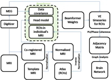
Fig. 1.Flow chart of analysis steps. The anatomical MRI is co-registered with the MEG and subsequently spatially normalised to a template MRI. Voxels in the template MRI are labelled using the Talairach Daemon Database. Voxels with the same label are

de-ﬁned as a ROI and transformed to the individual's co-registered MRI. The volume con-ductor model, based on the co-registered MRI, together with the data covariance created from selected time-frequency windows in the MEG data, is used to compute beamformer weights for the target locations in these ROIs. The MEG data are then pro-jected through the beamformer weights in order to create time-series (virtual elec-trodes) for these voxels. For each frequency band separately, a single time-series is constructed for each ROI (seeMethods) and the functional connectivity between the different ROIs is estimated by computing the Phase Lag Index (PLI) or Phase Coherence. Graph theory can subsequently be applied to the resulting adjacency matrix in order to characterise the functional network formed by the interacting ROIs (see Supplementa-ry material).

(4)

Assigning time-series to a ROI

Once the beamformer weights were estimated, Eq.(1)was used to reconstruct the time-series for each voxel. These virtual electrode time-series exhibit a non-uniform projection of sensor noise (the weights increase with depth, but the sensor level noise remains con-stant throughout the volume). In order to compensate for this inher-ent bias, we therefore normalise each beamformer weight by its vector norm before reconstructing the time-series (Cheyne et al., 2007).

A ROI in a subject's MRI contains several voxels, all with their own time-series (virtual electrodes). The direction of each estimated virtual electrode is arbitrary (a source pointing inwards with negative amplitude produces the same external magneticﬁeld as a source pointing outwards with positive amplitude), hence the estimated time-series for neighbour-ing virtual electrodes may have opposite polarities, renderneighbour-ing averagneighbour-ing of time-series across a ROI meaningless. We therefore proceeded to com-pute the spectrum for each virtual electrode time-series and divided the spectrum into the 5 classical EEG bands (delta (0.5–4 Hz), theta (4–

8 Hz), alpha (8–13 Hz), beta (13–30 Hz), and gamma (30–48 Hz)). For each ROI and frequency band separately, we selected the voxel with max-imum power in that frequency band, and used the time-series for this voxel for further analysis, resulting in a total of 5 sets of 68 time-series (one for each frequency band). Note that this procedure was carried out for each subject independently, such that the voxels that were selected to represent the ROIs were allowed to vary across subjects, mitigating the effects of co-registration, normalisation, and modelling errors (see e.g.Beal et al. (2010)for a similar strategy).

Estimating functional connectivity between ROIs

Functional interactions between sources of oscillatory activity can be captured by quantifying the phase relationship between their time-series (seePereda et al. (2005)for a review of coupling mea-sures). Unfortunately, despite the assumptions underlying beam-formers, the beamformer reconstructed sources may still show spurious,ﬁeld spread and volume conduction related, interactions, which manifests itself as locking with zero-phase lags. To show that this is the case, and to demonstrate how this problem can be solved, we use both Phase Coherence (PC) and PLI to estimate func-tional connectivity between ROIs.

The Phase Coherence quanti_ﬁes the phase coupling between two signals as follows (Mardia, 1972; Mormann et al., 2000):

PC¼

〈

eiΔφ

〉

¼ 1_SX S−1 k¼0 eiΔφð Þtk ; ð5Þ

whereΔΦis the phase difference between the instantaneous phases for the two time-series, deﬁned in the interval [0, 2π], tkare discrete

time-steps and S is the number of samples.

Phase Coherence captures consistent phase differences and is, un-like coherence, not inﬂuenced by the amplitude of the signals. Phase Coherence is maximal when the phase difference has a constant value, whatever the value of this phase difference is, and is therefore equally sensitive to both trivial (zero-phase) and true (zero-phase and nonzero-phase) interactions.

In contrast, the PLI is deﬁned as (Stam et al., 2007):

PLI¼

〈

sign sin½ ðΔφð ÞtkÞ

〉

; ð6Þ

where the phase difference is deﬁned in the interval [−π,π] andb> denotes the mean value. The PLI is non-zero when there is an asym-metry in the distribution of the instantaneous phase differences, and therefore only quantiﬁes non-trivial connections, at the expense of potentially discarding true interactions with zero-phase lag.

For the computation of the functional connectivity, using software developed by one of the authors (CS; Brainwave, version 0.8.92;

http://home.kpn.nl/stam7883/brainwave.html), 5 artefact-free data-segments of 4096 samples were selected from the ROI time-series after careful visual inspection.

For each ROI we computed the mean PLI and Phase Coherence with all other areas. This is also known as the weighted degree or node strength in terms of graph theory (Rubinov and Sporns, 2010), where individual values reﬂect the importance of nodes in the net-work, the mean across ROIs indicates the total‘wiring-cost’, and the distribution of degrees is an important marker of network develop-ment and resilience. We then computed the mean of this quantity across trials and subjects to get group mean node strength values per ROI.

Statistics

In order to determine the signiﬁcance of the empirical group mean values, we created 100 sets of null data by phase randomising (whilst maintaining the power spectra) the ROI time-series. For each realisa-tion, this gave rise to 68 new ROI time-series per subject, which were analysed in exactly the same way as the recorded data, giving a mean PLI value per ROI. Taking the maximum mean-PLI value over ROIs on each realisation gave a null distribution of PLI corrected for multiple comparisons across the volume.

Results

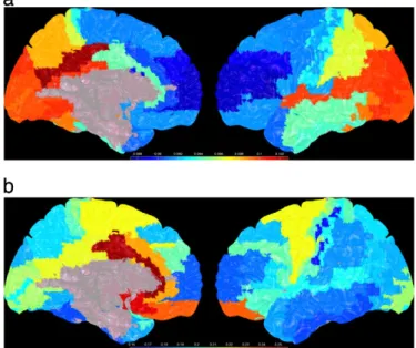
Fig. 2displays the mean functional connectivity for each ROI with all other ROIs. Note the differences between the maps for PLI and Phase Coherence, where Phase Coherence shows strongest functional connectivity for deeper structures, whereas the stron-gest PLI is found mainly for superﬁcial areas in the occipital and pa-rietal lobe and the superior temporal gyrus, as well as in the posterior cingulate.

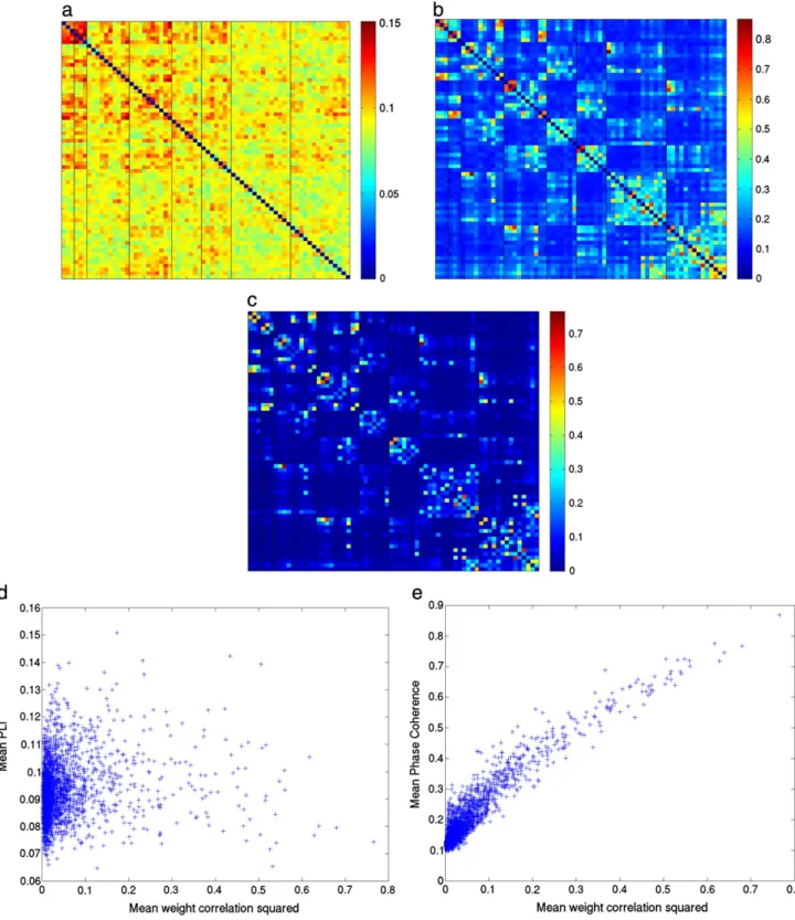
These differences can be explained by the different sensitivity of these measures to volume conduction/ﬁeld spread (in the form of correlation between beamformer weights). Fig. 3 shows that

Fig. 2.Mean PLI (upper panel) and mean Phase Coherence (lower panel) for the alpha band, displayed as a colour-coded map (unthresholded) on a schematic of the parcel-lated template brain.

(5)

there is a close correspondence between the weight correlations (Fig. 3c) and the Phase Coherence (Fig. 3b). This is conﬁrmed in

Fig. 3e, where a strong relationship between the weight correla-tions and Phase Coherence can be seen. This means that it is likely that any observed Phase Coherence could have been caused by

the beamformer itself. Such a clear relationship between the mean PLI and the weight correlations is not observable inFig. 3d.

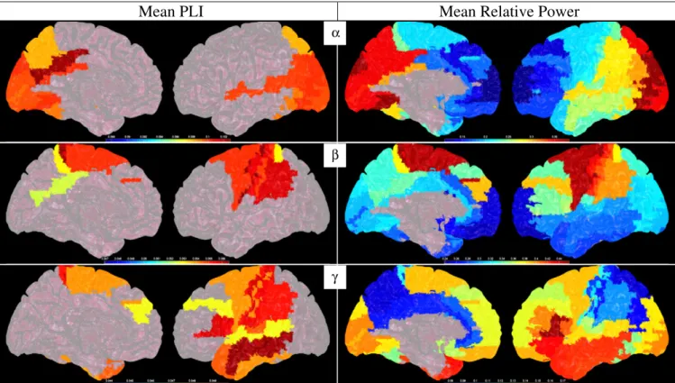
Fig. 4 displays the mean PLI for the alpha, beta and gamma bands (the adjacency matrices themselves are given in Supplemen-tary Fig. 1), as well as the mean relative power for these frequency

Fig. 3.Functional connectivity and relationship with the beamformer weights for the alpha band. a) Mean PLI adjacency matrix. The separation between anatomical groupings (from left to right: occipital, parietal/central, temporal, frontal) is denoted by a solid line, the separation between left and right hemisphere within each anatomical grouping is denoted by a dotted line (seeAppendix Afor details); b) mean Phase Coherence adjacency matrix; c) mean (squared) correlation between beamformer weights for each ROI (with the diagonal set to zero). Each element in this matrix was computed as follows: for each subject, the square of the correlation between the beamformer weights for a ROI and another ROI was computed. The mean over subjects of this value was then computed; d) Scatter plot of the (squared) correlation between beamformer weights and the PLI and (e) Phase Coherence.

(6)

bands. The mean PLI for the delta and theta bands did not reach sta-tistical signiﬁcance (see Supplementary Fig. 2 for the unthresholded PLI maps and maps of relative power for the delta and theta bands; Supplementary Fig. 3 shows results for the alpha1 and alpha2 bands).

The most strongly connected, as well as most strongly active, re-gions in the alpha band were the posterior cingulate, rere-gions in visual cortex and parietal lobe, as well as in the superior and inferior tempo-ral lobe.

The connectivity and power maps in the beta band showed a rel-atively restricted pattern of highly connected and strongly activated regions in the sensorimotor cortex, extending into the inferior parie-tal lobe and the dorsolateral prefronparie-tal cortex (for source power).

In the gamma band, the most strongly connected regions were in the temporal lobe, sensorimotor cortex and the inferior frontal and parietal lobes. Dominant power was also found in these regions, but covered more of the frontal lobe and also included the visual cortex, with notably less power in the parietal lobe and posterior part of the sensorimotor cortex.

It is clear fromFig. 4that the patterns for PLI and power are sim-ilar, but that there are also notable exceptions where regions with high power do not have corresponding high PLI values, and vice versa (compare for example the power and PLI values for the occipital pole and parietal lobe in the gamma band). This is further illustrated inFig. 5, where the relationship between PLI and power for the differ-ent frequency bands is shown. For all frequency bands, except the gamma band, there is a signiﬁcant positive linear relationship be-tween PLI and relative power (for delta, theta, alpha, beta and gamma bands respectively: F(1,66) = 69.98, pb10−11_{; F(1,66)}

= 8.99, pb0.01; F(1,66) = 194.31, pb10−15_; _{F(1,66) = 167.97,}

pb10−15; F(1,66) = 1.30,p= 0.26). However, the PLI values are not trivially related to the power values, as, for example, the relative power for the beta band and delta bands do not differ signiﬁcantly

(two-sample t(134) =−1.56,p= 0.12), whereas the mean PLI values are signiﬁcantly higher in the delta band than in the beta band (two-sample t(134) = 118.66,pb10−15_{). Similarly, the PLI for the theta and}

alpha bands do not differ signiﬁcantly (two-sample t(134) =−1.45,

p= 0.15), whereas the mean power values are signiﬁcantly higher in the alpha band than in the theta band (two-sample t(134) = 10.83,

pb10−15_).

Discussion and conclusions

We have presented a robust method for assessing significant func-tional connectivity across a group of subjects that is insensitive to volume conduction and statistically well controlled. Wefirst demonstrated that when using Phase Coherence, functional connectivity estimates, even at the source-level, are biased due to the effects of volume conduction andfield spread. In contrast, functional connectivity estimates based on PLI are not affected by these biases. Subsequently, we used the method to show significantly higher than chance interactions between regions in three of the five frequency bands studied, revealing distinct frequency-band dependent patterns of functional connectivity across the brain.

Alpha band

Strong connectivity was observed in the visual cortex and in the pa-rietal and temporal lobes, consistent with theﬁndings byGuggisberg et al. (2008). However, we could notﬁnd any direct evidence in the exist-ing literature for the strong restexist-ing-state functional connectivity in the posterior cingulate for the alpha band.

Similarly, the dominant alpha power in the posterior part of the brain is consistent with the established patterns of eyes-closed resting-state alpha activity (e.g.Pfurtscheller, 1992; Rosanova et al., 2009). Additionally, several studies, using different methodologies

α

β

γ

Mean PLI

Mean Relative Power

Fig. 4.Mean PLI (left column, thresholded at p = 0.05) and mean relative power (right column) for alpha, beta and gamma bands (top to bottom), displayed as a colour-coded map on a schematic of the parcellated template brain (see Supplementary Fig. 4 for unthresholded results). SeeAppendix Bfor a list of the areas with signiﬁcant mean PLI.

(7)

and modalities, have reported activations similar to ours for the visual cortex, parietal and temporal lobe (Congedo et al., 2010; Srinivasan et al., 2006) as well as the posterior cingulate (Congedo et al., 2010).

Beta band

We found strong resting-state beta-band functional connectivity in the sensorimotor cortex, in agreement with a previous MEG resting-state functional connectivity study (Brookes et al., 2011a). Moreover, the large body of literature on beta-band synchrony in sen-sorimotor systems involved in co-ordinated movement and posture (e.g.Farmer, 1998), suggests that these systems are also connected in this frequency band during rest. Further evidence for this hypoth-esis comes from single-pulse TMS studies that have shown that TMS synchronises the phase of beta-oscillations (van der Werf and Paus, 2006; van der Werf et al., 2006), and that stimulating one region of the sensorimotor system can induce activity in another part of this system (e.g.Caramia et al., 2000).

Ourﬁnding of strong resting-state beta power in sensori-motor cor-tex and inferior parietal lobe is consistent with studies that have revealed event-related beta-power reductions in these regions follow-ing somatosensory stimulation or movement (e.g.Gaetz and Cheyne, 2006; Jurkiewicz et al., 2006; Maratos et al., 2007; Taniguchi et al., 2000), or that showed that the beta-band is the natural frequency of these circuits (Rosanova et al., 2009). Our observed beta band power in the dorsolateral prefrontal cortex can tentatively be related to the reorienting of attention (Altamura et al., 2010).

Gamma band

We had naively expected that gamma band PLI (like alpha band PLI) would predominate in the visual cortex. We found little litera-ture to corroborate the resting-state functional connectivity in the temporal lobe, sensorimotor cortex and the inferior frontal and parietal lobe for the gamma band. Recent invasive electrode (Grifﬁths et al., 2010) and non-invasive studies on pitch perception (Sedley et al., 2012) have pointed to a functional role for the gamma band in the region of human auditory cortex. It would

make sense that similar functional units are also to some degree engaged during the resting-state.

In terms of source power however, the observed dominant power in the frontal and temporal lobe is in agreement with previous EEG

ﬁndings (Chen et al., 2008). Our observations are also in agreement with reports of both resting-state measures of gamma power in the primate (Leopold and Logothetis, 2003) and event-related changes in gamma power in visual cortex following visual stimulation (e.g.

Adjamian et al., 2004; Hall et al., 2005b, 2005a; Hoogenboom et al., 2006).

Relationship between source power and functional connectivity

We found a positive relationship between the patterns of source power and functional connectivity, using a connectivity measure that is not sensitive to power or volume conduction. The fact that we found this relationship for all frequency bands (except the gamma band) suggests that there may be a general mechanism that explains this relationship. The simplest explanation is that a positive relationship between source power and connectivity was introduced by our analysis approach, since the functional connectivity measure that we used relies on accurate estimation of phase differences, and therefore on a high-enough SNR. Consequently, functional connectiv-ity between regions with low source power may be missed or under-estimated, introducing a bias towards a positive correlation between power and connectivity. However, we didfind regions with strong connections despite low source power (e.g. parietal lobe for the gamma band,Fig. 4), hence it is unlikely that the positive relationship between source power and connectivity can be fully explained by such a methodological bias. One possible physiological mechanism that could provide an alternative explanation has been identified through modelling studies (Chawla et al., 1999, 2000), which have shown that increased mean spiking activity within two connected neuronal populations leads to increased intra- and interregional phase locking, or in other words, to simultaneous increases in power and functional connectivity. This coupling between functional connectivity and mean activity was mainly achieved through a reduc-tion in mean membrane integrareduc-tion times as activity increased, which then introduced a bias towards synchronousfiring (Chawla et al., 1999). Recent modelling work has also shown an amplitude depen-dency of interregional phase locking, albeit that this dependepen-dency was more complex (Daffertshofer and van Wijk, 2011).

Methodological considerations General analysis framework

A frequent criticism of sensor-level connectivity/network analysis is that the results are biased by the effects of volume conduction/ﬁeld spread (Schoffelen and Gross, 2009). Our results show that this prob-lem is not completely solved by going to source-space (Fig. 3), as it reveals itself, in our case, in the form of correlation between beamfor-mer weights. As a solution, we used the PLI, which quantiﬁes func-tional interactions that are not caused by volume conduction or common sources. The main reason for going to the source-level, in combination with an atlas-based analysis approach, is therefore that it provides a general framework that allows for a direction anatomical interpretation of MEG data, as well as a direct comparison with (functional) connectivity and network studies based on anatomical MRI (Diffusion Tensor Imaging, Voxel-based Morphometry) and func-tional MRI (e.g.Gong et al., 2009; van den Heuvel and Hulshoff Pol, 2010). We envisage that the understanding of resting-state networks will be much enhanced by such a combination of different modalities. Similarly, our approach enables the integration and direct comparison of data recorded with different MEG systems. Although we have focussed here on the eyes-closed resting-state, our approach can also be applied to compare patterns of oscillatory activity and functional networks for different cognitive states.

Fig. 5.Mean PLI versus mean relative power for the different frequency bands. Note that there is a signiﬁcant positive linear relationship between PLI and relative power, for all frequency bands, except the gamma band. Also note that, for each frequency band separately, the mean PLI varies over only a limited range, and that the variance in PLI that can be explained by source power is relatively small (R2_{= 51%, 12%, 75%,} 72% and 2% for the delta, theta, alpha, beta and gamma bands respectively).

(8)

One can consider the choice of using a set of atlas-based ROIs as a compromise between all-to-all connectivity estimates (Schoffelen and Gross, 2011) and methods based on a-priori selection of a small number of regions (Astolfiet al., 2007; Friston et al., 2011; Siegel et al., 2008). The use of atlas-based ROIs does certainly compromise the potential spatial resolution, but could be the most ef_ficient level of description given the inter-individual variability. Similarly, the use of predefined anatomical regions does mean that one samples from all sources rather than just those with highest source power (al-though within each ROI we did select the voxel with highest source power), thereby avoiding the danger that weakly activated, but strongly interacting, sources are missed (compare for example the connectivity and power in the parietal lobe for the gamma band (Fig. 4)).

Choice of source reconstruction approach

We chose to reconstruct the resting-state sources, and their time-series, using a beamforming approach, as this approach does not suf-fer from the problems associated with linear inverse solutions (wide-spread correlations between reconstructed source elements and problematic interpretation of reconstructed images of source power). A potential limitation of the beamformer-based approach is that the beamformer weights are based on source power and interacting sources with small amplitude could therefore be missed (but see

Fig. 4, gamma band power and connectivity). Moreover, the beamfor-mer weights are designed so that the sensitivity to signals from a lo-cation of interest is increased, whilst reducing the contribution of signals from (noise) sources at different locations. As a consequence the contribution from sources that are perfectly linearly correlated is cancelled or underestimated (which might in particular be prob-lematic for weak long-distance interactions). Atﬁrst sight, this prop-erty of beamforming seems therefore at odds with our aim to estimate interactions between sources. However, there are several reasons why beamforming can still be applied in studies on functional connectivity: i) it is important to stress that only (zero-lag) linearly correlated sources are problematic for the beamformer. Non-linear measures of functional connectivity should therefore be less affected; ii) even for linearly correlated sources, there is a remarkable tolerance to deviations from the uncorrelatedness-assumption, such that source interdependencies can be accurately reconstructed even when these sources are correlated for 30–40% of the analysis time-window (Hadjipapas et al., 2005); iii) anatomical and electrophysio-logical data suggest that the uncorrelatedness-assumption is plausible (Hillebrand and Barnes, 2005); and iv) modiﬁed beamformer ap-proaches are available to deal with those rare cases where sources with strong linear interactions are present (Brookes et al., 2007; Dalal et al., 2006; Diwakar et al., 2011; Hui et al., 2010; Quraan and Cheyne, 2010). In addition, the PLI and beamformer blindspots sit comfortably together—the beamformer will potentially mis-localise sources with zero-lag correlation but by using the PLI we ignore these effects.

Other methods, such as minimum norm based approaches, have no such constraints on source correlation. However, thisﬂexibility comes at the price of poorer noise rejection capability. The work of Ghuman et al. highlights the problems that occur when combining a minimum norm approach with aphase-locking(rather than phase-lagging) approach, in that one has to rely on the subtraction of empty room data in order to try to remove the large number of spu-rious interactions (Ghuman et al., 2011). A particular worry here is that minimum norm based source reconstruction approaches inher-ently model all the data and therefore project artefacts (such as heart-beat or from external noise sources) into the source space. In contrast, beamforming approaches only localise those components in the data that match the leadﬁeld for a source at a particular location, giving beamformers the ability to reject artefacts (e.g. Adjamian et al., 2009). Importantly, these projected artefacts lead to further spurious

connectivity estimates when using methods that are sensitive to zero-phase interactions (i.e. methods based on phase-locking, rather than PLI).

Beamformer implementations exist that use the matrix of connec-tions (Gross et al., 2001) or higher order statistics (Huang et al., 2004), rather than the data covariance matrix, for the computation of the beamformer weights (Eq.(2)). One could also consider the di-rect replacement of the data covariance matrix by the PLI adjacency matrix when computing the beamformer weights, thereby avoiding problems related to volume conduction and zero-lag phase relations between sources. This may be problematic though, since the PLI is in-dependent of signal amplitude. However, further research could show whether the use of the imaginary coherence, which also minimises the inﬂuence of volume conduction, proves to be more fruitful in this type of approach.

Selection of ROIs

We chose to parcellate the source space on the basis of the Talair-ach Daemon Database, although alternative atlases are available (e.g.

Collins et al., 1995; Tzourio-Mazoyer et al., 2002). Instead, one could also use a parcellation-scheme that is based on the source-sensor ge-ometry in order to obtain a set of maximally independent patches (Palva et al., 2010a), or perform parcellation in the native MRIs (Seibert and Brewer, 2011). This latter option would in particular be preferably for patients who's MRI match poorly to a template MRI, for example due to atrophy. In addition, it remains an open question how best to deal with ROIs of unequal size. One could argue that all ROIs should contain an equal number of voxels so that estimates of interdependencies are not affected by differences in ROI size. In con-trast, perhaps the size of a ROI should reﬂect the variations in sensi-tivity of MEG to neuronal acsensi-tivity in different regions of the brain (Hillebrand and Barnes, 2002). Overall, these disadvantages of using a standard brain-atlas are outweighed by the important advantage that its use enables a more direct comparison between data from dif-ferent modalities (Plis et al., 2011).

Beamformer weight estimation

Here, we used the beamformer formulation for point sources, i.e. the leadfields for equivalent current dipoles were used for the weight computations. In order to take into account the spatial extent of the ROIs for which representative time-series are estimated, one could use the leadfields for spatially extended sources (Hillebrand and Barnes, 2011), use a set of basis functions (Limpiti et al., 2004, 2006), or use Singular Value Decomposition (SVD) to define a lower-dimensional representation for each ROI (Gross and Ioannides, 1999). Similarly, a combination of Signal Space Separation (SSS) and beamforming allows for the estimation of time-series for pre-defined spherical ROIs (Ozkurt et al., 2009), although with this approach one would lose the advantages of using a standard brain atlas. Instead, the direct replacement of the SAM beamformer by the recently developed SSS-beamformer (Vrba et al., 2010) would fit more naturally in our proposed analysis framework.

Recently,Hui et al. (2010)have proposed a nulling-beamformer, which removes potential cross-talk between ROIs by incorporating additional (nulling-) constraints for these ROIs into the beamfor-mer design. It is not clear though how the reduction in the degrees of freedom due to the use of many ROIs in a standard atlas (i.e. many nulling-constraints would be needed) would affect both the ability to reject noise and the accuracy of the reconstructed time-series.

We used a multi-sphere head model for the computation of the lead

ﬁelds, which provides an accurate approximation of the volume conduc-tor for MEG (Huang et al., 1999), although more complex numerical models may provide increased accuracy in certain situations (Lalancette et al., 2011). Inaccuracies in the volume conductor model may lead to underestimation of source power (Hillebrand and Barnes,

(9)

2003, 2005). However, given that PLI is independent of amplitude, it is unlikely that connectivity biases were introduced, even if there were re-gions for which source power was underestimated.

The length of the data covariance window that was used for the weight computations was determined by the amount of data that was available from each recording session, the duration of which was set at what was common practice for a resting-state MEG session at the time of recording (2003/2004). Simulation studies have shown that the required number of samples for beamforming depends, among other factors, on the frequency-band of interest, sampling rate and source power (Brookes et al., 2008). The results by Brookes et al. suggest that even for our worst case scenario (small band width of 3.5 Hz for the delta band and smallest co-variance window of 175 s) the errors in the estimation of the data covariance, and therefore in source power estimates, were minimal (less than 10% un-derestimation in source power).

It is feasible to apply noise-regularisation during the compu-tation of the beamformer weights (not used in this study), which would lead to increased signal-to-noise ratio (SNR) for the estimated time-series, and would also mitigate against the effects of using a limited set of (atlas-based) voxels in template space (activation could be missed due to co-registration and nor-malisation errors—see e.g.Beal et al. (2010)for a similar strate-gy). However, regularisation comes at the expense of a decreased ability to distinguish spatially separate sources (Gross and Ioannides, 1999). The optimal trade-off between this temporal and spatial accuracy for studies that aim to compute the topogra-phy and topology of functional networks, has yet to be deter-mined for empirical data.

Deﬁning representative time-series for a ROI

To deal with the issue of arbitrary sign for the orientation of the source at each voxel, which makes straightforward averaging of source waveforms across a ROI impossible, we selected the voxel with maximum source power within a ROI. It has been shown previ-ously (Barnes et al., 2004) that the time-series estimated at local maxima best describe the underlying source activity. For datasets with large artefacts, these artefacts could leak into the reconstructed time-series and potentially bias the selection of the voxel with maxi-mum power. Alternative approaches include: i) performing a check on (and adjustment of) the polarity of the time-series of neighbouring voxels before averaging time-series across a ROI. This assumes that the source orientation varies smoothly when moving through the source space; ii) using SVD toﬁnd the eigenvectors (time-series) that best rep-resent the time-series of the ROI (see e.g.Supp et al., 2007); and iii) using the series that most strongly correlates with the time-series for the other voxels in the ROI.

A consequence of selecting the voxels with maximum power to represent the ROIs is that, particularly when source activation spreads over multiple ROIs, the peak voxels for neighbouring ROIs can be close together (Supplementary Fig. 5), i.e. such voxels share (almost) the same signal. For such cases, the source reconstruction approach could not unambiguously determine whether the activity is coming from one or the other ROI (or both). Importantly, PLI is insensitive to the spurious zero-lag interactions that could exist between voxels that are close together, hence the voxel selection will not lead to overestimates of (local) connectivity.

Alternatively, one could, for each voxel, extract the power mod-ulations of the time-series using the Hilbert transform (Byron and Fuller, 1992) and average these envelopes across a ROI. This ap-proach has already demonstrated interesting relationships between functional networks constructed on the basis ofﬂuctuations in MEG band-limited power and those based on low-frequency modulations in BOLD fMRI time-series (Liu et al., 2010). A limitation of this approach is that differences in ROI size might result in biases due to differences in SNR.

Connectivity estimation

In this work we contrasted PLI with Phase Coherence as mea-sures of functional connectivity between ROIs. As expected, the Phase Coherence suffers from spurious correlations between ROIs due to correlations between their beamformer weights (Fig. 3). PLI on the other hand is a conservative measure that is insensitive to such spurious interactions, albeit at the expense that true zero-lag correlations are also missed. Zero-zero-lag correlations are most-likely to be short-range (e.g.Gray et al., 1989), but see (Rodriguez et al., 1999; Roelfsema et al., 1997; Tognoli and Kelso, 2009; Vicente et al., 2008), and functional networks constructed on the basis of PLI could therefore have a topology for which the clustering and/or modularity are underestimated. Note that this is a general issue for all MEG/EEG connectivity studies, and not a problem that is speciﬁc for the proposed analysis framework. In fact, when im-proved connectivity estimators become available, then they can easily be incorporated in our analysis framework. Vinck et al. (2011)have recently described a promising modiﬁcation of PLI with reduced underestimation of connectivity between sources with small-lag interactions, as well as a reduced estimator bias, although this comes at the expense of introducing an arbitrary bias favouring large phase differences and mixing of the estimation of consistency of phase differences with the estimation of the magnitude of the phase difference. An alternative approach that would avoid these issues, and at the same time reduce the effects of noise on PLI-based connectivity estimates (par-ticularly when interactions occur with almost zero-phase lag) would be to ignore phase differences within a small window around zero and around ±π. However, although the use of such an offset could potentially be useful when considering small numbers of trials, noise-related counts of positive and negative phase lags (regardless of magnitude) should not bias the statistics.

We should note that the time window for the connectivity anal-ysis was ﬁxed here at 13.1 s, and that we analysed 5 of such artefact-free data-segments. Clearly, the choice of time window de-termines not only the expected period of stationarity of the interac-tions, but also the bandwidth over which interactions can occur. Further investigations may reveal whether different forms of inter-actions are highlighted for different choices of time-frequency pa-rameters. Indeed, empirical observations have revealed that relatively short epochs (~ 10 s) are quasi-stationary, and that such short epochs can already be representative of a subject's cognitive

ﬁngerprint (seeSchomer and Lopes da Silva, 2010). Moreover, the work byHoney et al. (2007)has shown that functional networks at these time-scales are stable yet dynamic (on longer time-scales the functional networks resemble the underlying (static) anatomi-cal network, whereas on shorter timesanatomi-cales the functional net-works are highly variable). Additionally, it has been shown that using 5 epochs of 10 s resting-state data results in fairly good to good levels of test–retest reliabilities, depending on the frequency band and metrics analysed (Jin et al., 2011). It should be noted that Lin et al. analysed magnetometer data at the sensor level and computed complex network metrics, whereas in our study third-order gradiometer data was analysed using a beamformer ap-proach, both resulting in improved SNR, and that we used simple metrics to characterise the functional networks; these factors all contribute to an increased stability of the estimated resting-state network properties (Deuker et al., 2009; Jin et al., 2011). Finally, using the same number of epochs as we routinely use in our clinical studies, which has proven to give stable estimates of resting-state activity/network parameters (e.g.Douw et al., 2011), renders our developed methodology and the results from the current study di-rectly relevant to our clinical work.

We looked at the average overall connectivity for a ROI, not, as is typical in fMRI, speciﬁcally at connections between certain ROIs. For example, the average connectivity for a ROI could be relatively low, but the ROI could still have strong connections with (only) some

(10)

ROIs in, let's say, the default mode network. A more in depth com-parison with the fMRI literature would be an interesting topic for fu-ture research. Indeed, recent work (Brookes et al., 2011b) has shown the correspondence between beamformer estimated power envelope correlations and fMRI deﬁned resting-state networks. It will be interesting to see the make-up of the fMRI de_ﬁned networks in terms of the relative contributions of electrical interactions over dimensions of power, phase and frequency.

Statistics

For the creation of the phase-randomised surrogates we did not take into account any jumps at the boundaries, which could have introduced high-frequency artefacts in our surrogate data (Kantz and Schreiber, 1997). However, any biases introduced in our statistics will have been minimal, as we subsequentlyﬁltered the surrogate data to relatively low frequencies (maximal 48 Hz for the gamma band).

We have introduced a general MEG analysis framework for the reconstruction of frequency-dependent proﬁles of source power and functional connectivity, which is robust to artefactual connec-tivity estimates caused by volume conduction, due to the use of the PLI; robust to artefactual connectivity estimates caused by physiological (e.g. heartbeat) and environmental (e.g. power-line) noise, due to the use of the beamformer approach; robust to co-registration errors, due to the use of unconstrained source

orientation at each voxel; and robust to modelling errors (e.g. intro-duced by co-registration errors or by ignoring source extent), due to the use of coarse spatial sampling (de_ﬁned by the ROIs). Finally, the results are based on non-parametric statistics with few under-lying assumptions.

The analysis framework contains two important elements: i) ac-tivity is reconstructed for an atlas-based set of ROIs in order to facil-itate interpretation and comparison with results obtained with other modalities; and ii) effects of volume conduction/ﬁeld spread on estimated interactions between ROIs are removed using PLI, a measure that is insensitive to these effects. Using this framework we have revealed distinct frequency-dependent patterns of source power and source interactions. We envisage that this approach will be used to further elucidate the patterns of resting-state activ-ity in health and disease (Fox and Greicius, 2010; Guggisberg et al., 2008; Martino et al., 2011; Ortega et al., 2008).

Supplementary materials related to this article can be found online atdoi:10.1016/j.neuroimage.2011.11.005.

Acknowledgments

This study was supported by a grant from the Royal Society (Inter-national Joint Projects 2007/R1), which was awarded whilst AH and GRB were at Aston University. The WTCN is supported by a strategic award from the Wellcome Trust. The authors also thank Krish Singh for support with the labelling of ROIs.

Appendix A

Appendix B

List of the Brodmann areas, and the labels, that were used. L denotes left hemisphere, R denotes right hemisphere. For the display of the adjacency matrices, the following groupings were deﬁned based on the indices in this table: left occipital (7, 9, 11), right occipital (8, 10, 12), left parietal/central (1, 13, 27, 59, 63, 39, 43, 49, 29, 21), right parietal/central (2, 14, 28, 60, 64, 40, 44, 50, 30, 22), left temporal (45, 47, 19, 17, 15, 35, 37), right temporal (46, 48, 20, 18, 16, 36, 38), left frontal (41, 61, 65, 67, 3, 55, 53, 51, 5, 57, 25, 31, 23, 33), right frontal (42, 62, 66, 68, 4, 56, 54, 52, 6, 58, 26, 32, 24, 34).

Index ROI label Index ROI label

1 BA 1: primary somatosensory cortex (L) 35 BA 37: fusiform gyrus (L) 2 BA 1: primary somatosensory cortex (R) 36 BA 37: fusiform gyrus (R) 3 BA 10: anterior prefrontal cortex (L) 37 BA 38: temporopolar area (L) 4 BA 10: Anterior prefrontal cortex (R) 38 BA 38: temporopolar area (R) 5 BA 11: orbitofrontal cortex (L) 39 BA 39: angular gyrus (L) 6 BA 11: orbitofrontal cortex (R) 40 BA 39: angular gyrus (R) 7 BA 17: primary visual cortex (L) 41 BA 4: primary motor cortex (L) 8 BA 17: primary visual cortex (R) 42 BA 4: primary motor cortex (R) 9 BA 18: secondary visual cortex (L) 43 BA 40: supramarginal gyrus (L) 10 BA 18: secondary visual cortex (R) 44 BA 40: supramarginal gyrus (R)

11 BA 19: associative visual cortex (L) 45 BA 41: primary and auditory association cortex (L) 12 BA 19: associative visual cortex (R) 46 BA 41: primary and auditory association cortex (R) 13 BA 2: primary somatosensory cortex (L) 47 BA 42: primary and auditory association cortex (L) 14 BA 2: primary somatosensory cortex (R) 48 BA 42: primary and auditory association cortex (R) 15 BA 20: inferior temporal gyrus (L) 49 BA 43: primary gustatory cortex (L)

16 BA 20: inferior temporal gyrus (R) 50 BA 43: primary gustatory cortex (R) 17 BA 21: middle temporal gyrus (L) 51 BA 44: pars opercularis (L) 18 BA 21: middle temporal gyrus (R) 52 BA 44: pars opercularis (R) 19 BA 22: superior temporal gyrus (L) 53 BA 45: pars triangularis (L) 20 BA 22: superior temporal gyrus (R) 54 BA 45: pars triangularis (R)

21 BA 23: ventral posterior cingulate (L) 55 BA 46: dorsolateral prefrontal cortex (L) 22 BA 23: ventral posterior cingulate (R) 56 BA 46: dorsolateral prefrontal cortex (R) 23 BA 24: ventral anterior cingulate (L) 57 BA 47: inferior prefrontal gyrus (L) 24 BA 24: ventral anterior cingulate (R) 58 BA 47: inferior prefrontal gyrus(R) 25 BA 25: ventromedial prefrontal cortex (L) 59 BA 5: somatosensory association cortex (L) 26 BA 25: ventromedial prefrontal cortex (R) 60 BA 5: somatosensory association cortex (R)

27 BA 3: primary somatosensory cortex (L) 61 BA 6: premotor cortex and supplementary motor area (L) 28 BA 3: primary somatosensory cortex (R) 62 BA 6: premotor cortex and supplementary motor area (R) 29 BA 31: dorsal posterior cingulate cortex (L) 63 BA 7: somatosensory association cortex (L)

30 BA 31: dorsal posterior cingulate cortex (R) 64 BA 7: somatosensory association cortex (R) 31 BA 32: dorsal anterior cingulate cortex (L) 65 BA 8: frontal cortex including frontal eyeﬁelds (L) 32 BA 32: dorsal anterior cingulate cortex (R) 66 BA 8: frontal cortex including frontal eyeﬁelds (R) 33 BA 33: anterior cingulate cortex (L) 67 BA 9: dorsolateral prefrontal cortex (L)

(11)

References

Adjamian, P., Holliday, I.E., Barnes, G.R., Hillebrand, A., Hadjipapas, A., Singh, K.D., 2004. Induced visual illusions and gamma oscillations in human primary visual cortex. Eur. J. Neurosci. 20, 587–592.

Adjamian, P., Worthen, S.F., Hillebrand, A., Furlong, P.L., Chizh, B.A., Hobson, A.R., Aziz, Q., Barnes, G.R., 2009. Effective electromagnetic noise cancellation with beamformers and synthetic gradiometry in shielded and partly shielded environments. J. Neurosci. Methods 178, 120–127.

Altamura, M., Goldberg, T.E., Elvevag, B., Holroyd, T., Carver, F.W., Weinberger, D.R., Cop-pola, R., 2010. Prefrontal cortex modulation during anticipation of working memory demands as revealed by magnetoencephalography. Int. J. Biomed. Imaginghttp:// www.hindawi.com/journals/ijbi/2010/840416/.

Arieli, A., Sterkin, A., Grinvald, A., Aertsen, A., 1996. Dynamics of ongoing activity: explanation of the large variability in evoked responses. Science 273, 1868–1871. Astolﬁ, L., Cincotti, F., Mattia, D., Marciani, M.G., Baccala, L.A., de Vico, F.F., Salinari, S., Ursino, M., Zavaglia, M., Ding, L., Edgar, J.C., Miller, G.A., He, B., Babiloni, F., 2007. Comparison of different cortical connectivity estimators for high-resolution EEG recordings. Hum. Brain Mapp. 28, 143–157.

Babiloni, F., Cincotti, F., Babiloni, C., Carducci, F., Mattia, D., Astolﬁ, L., Basilisco, A., Rossini, P.M., Ding, L., Ni, Y., Cheng, J., Christine, K., Sweeney, J., He, B., 2005. Estimation of the cortical functional connectivity with the multimodal integration of high-resolution EEG and fMRI data by directed transfer function. Neuroimage 24, 118–131. Barnes, G.R., Hillebrand, A., 2003. Statisticalﬂattening of MEG beamformer images.

Hum. Brain Mapp. 18, 1–12.

Barnes, G.R., Hillebrand, A., Fawcett, I.P., Singh, K.D., 2004. Realistic spatial sampling for MEG beamformer images. Hum. Brain Mapp. 23, 120–127.

Bassett, D.S., Meyer-Lindenberg, A., Achard, S., Duke, T., Bullmore, E., 2006. Adaptive reconﬁguration of fractal small-world human brain functional networks. Proc. Natl. Acad. Sci. U.S.A. 103, 19518–19523.

Beal, D.S., Cheyne, D.O., Gracco, V.L., Quraan, M.A., Taylor, M.J., De Nil, L.F., 2010. Auditory evokedﬁelds to vocalization during passive listening and active genera-tion in adults who stutter. Neuroimage 52, 1645–1653.

Born, R.T., Bradley, D.C., 2005. Structure and function of visual area MT. Annu. Rev. Neurosci. 28, 157–189.

Bosboom, J.L., Stoffers, D., Stam, C.J., van Dijk, B.W., Verbunt, J., Berendse, H.W., Wolters, E.C., 2006. Resting state oscillatory brain dynamics in Parkinson's disease: an MEG study. Clin. Neurophysiol. 117, 2521–2531.

Bosboom, J.L., Stoffers, D., Wolters, E.C., Stam, C.J., Berendse, H.W., 2009. MEG resting state functional connectivity in Parkinson's disease related dementia. J. Neural Transm. 116, 193–202.

Brookes, M.J., Stevenson, C.M., Barnes, G.R., Hillebrand, A., Simpson, M.I., Francis, S.T., Morris, P.G., 2007. Beamformer reconstruction of correlated sources using a modiﬁed source model. Neuroimage 34, 1454–1465.

Brookes, M.J., Vrba, J., Robinson, S.E., Stevenson, C.M., Peters, A.M., Barnes, G.R., Hillebrand, A., Morris, P.G., 2008. Optimising experimental design for MEG beamformer imaging. Neuroimage 39, 1788–1802.

Brookes, M.J., Hale, J.R., Zumer, J.M., Stevenson, C.M., Francis, S.T., Barnes, G.R., Owen, J.P., Morris, P.G., Nagarajan, S.S., 2011a. Measuring functional connectivity using MEG: methodology and comparison with fcMRI. Neuroimage 56, 1082–1104. Brookes, M.J., Woolrich, M., Luckhoo, H., Price, D., Hale, J.R., Stephenson, M.C., Barnes, G.R.,

Smith, S.M., Morris, P.G., 2011b. Investigating the electrophysiological basis of resting state networks using magnetoencephalography. Proc. Natl. Acad. Sci. U.S.A. 108, 16783–16788.

Byron, F.W., Fuller, R.W., 1992. Mathematics of Classical and Quantum Physics. Dover Publications, Mineola.

Caramia, M.D., Palmieri, M.G., Giacomini, P., Iani, C., Dally, L., Silvestrini, M., 2000. Ipsilateral activation of the unaffected motor cortex in patients with hemiparetic stroke. Clin. Neurophysiol. 111, 1990–1996.

Chawla, D., Lumer, E.D., Friston, K.J., 1999. The relationship between synchronization among neuronal populations and their mean activity levels. Neural Comput. 11, 1389–1411. Chawla, D., Lumer, E.D., Friston, K.J., 2000. Relating macroscopic measures of brain

activity to fast, dynamic neuronal interactions. Neural Comput. 12, 2805–2821. Chen, A.C., Feng, W., Zhao, H., Yin, Y., Wang, P., 2008. EEG default mode network in the

human brain: spectral regionalﬁeld powers. Neuroimage 41, 561–574. Cheung, B.L., Riedner, B.A., Tononi, G., van Veen, B.D., 2010. Estimation of cortical

connec-tivity from EEG using state-space models. IEEE Trans. Biomed. Eng. 57, 2122–2134. Cheyne, D., Bostan, A.C., Gaetz, W., Pang, E.W., 2007. Event-related beamforming: a

robust method for presurgical functional mapping using MEG. Clin. Neurophysiol. 118, 1691–1704.

Collins, D.L., Holmes, C.J., Peters, T.M., Evans, A.C., 1995. Automatic 3-D model-based neuroanatomical segmentation. Hum. Brain Mapp. 3, 190–208.

Congedo, M., John, R.E., De, R.D., Prichep, L., 2010. Group independent component analysis of resting state EEG in large normative samples. Int. J. Psychophysiol. 78, 89–99. Daffertshofer, A., van Wijk, B.C., 2011. On the inﬂuence of amplitude on the connectivity

between phases. Front Neuroinform. 5, 6.

Dalal, S.S., Sekihara, K., Nagarajan, S.S., 2006. Modiﬁed beamformers for coherent source region suppression. IEEE Trans. Biomed. Eng. 53, 1357–1363.

David, O., Garnero, L., Cosmelli, D., Varela, F., 2002. Estimation of neural dynamics from MEG/EEG cortical current density maps: application to the reconstruction of large-scale cortical synchrony. IEEE Trans. Biomed. Eng. 49, 975–987.

David, O., Cosmelli, D., Lachaux, J.P., Baillet, S., Garnero, L., Martinerie, J., 2003. A theo-retical and experimental introduction to the non-invasive study of large-scale neural phase synchronization in human beings. Int. J. Comput. Cogn. 1, 53–77. de Pasquale, F., Della Penna, S., Snyder, A.Z., Lewis, C., Mantini, D., Marzetti, L., Belardinelli,

P., Ciancetta, L., Pizzella, V., Romani, G.L., Corbetta, M., 2010. Temporal dynamics of spontaneous MEG activity in brain networks. Proc. Natl. Acad. Sci. U.S.A. 107, 6040–6045.

De Vico Fallani, F., Astolﬁ, L., Cincotti, F., Mattia, D., Marciani, M.G., Salinari, S., Kurths, J., Gao, S., Cichocki, A., Colosimo, A., Babiloni, F., 2007. Cortical functional connectivity networks in normal and spinal cord injured patients: evaluation by graph analysis. Hum. Brain Mapp. 28, 1334–1346.

Deuker, L., Bullmore, E.T., Smith, M., Christensen, S., Nathan, P.J., Rockstroh, B., Bassett, D.S., 2009. Reproducibility of graph metrics of human brain functional networks. Neuroimage 47, 1460–1468.

Ding, L., Worrell, G.A., Lagerlund, T.D., He, B., 2007. Ictal source analysis: localization and imaging of causal interactions in humans. Neuroimage 34, 575–586. Diwakar, M., Tal, O., Liu, T.T., Harrington, D.L., Srinivasan, R., Muzzatti, L., Song, T., Theilmann,

R.J., Lee, R.R., Huang, M.X., 2011. Accurate reconstruction of temporal correlation for neuronal sources using the enhanced dual-core MEG beamformer. Neuroimage 56, 1918–1928.

Domínguez, L.G., Wennberg, R., Velázquez, J.L.P., Erra, R.G., 2007. Enhanced measured synchronization of unsynchronized sources: inspecting the physiological signiﬁ -cance of synchronization analysis of whole brain electrophysiological recordings. Int. J. Phys. Sci. 2, 305–317.

Dossevi, A., Cosmelli, D., Garnero, L., Ammari, H., 2008. Multivariate reconstruction of functional networks from cortical sources dynamics in MEG/EEG. IEEE Trans. Biomed. Eng. 55, 2074–2086.

Ranked list of the Brodmann areas that had signiﬁcant (pb0.05) mean PLI with all other ROIs. BA denotes Brodmann area, L denotes left hemisphere, R denotes right hemisphere.

Alpha Beta Gamma

BA 31: dorsal posterior cingulate (R) BA 4: primary motor (L) BA 21: middle temporal gyrus (R) BA 19: associative visual (R) BA 40: supramarginal gyrus (L) BA 3: primary somatosensory (R) BA 23: ventral posterior cingulate (L) BA 3: primary somatosensory (L) BA 45: pars triangularis (R) BA 23: ventral posterior cingulate (R) BA 1: primary somatosensory (L) BA 41: primary auditory (R) BA 39: angular gyrus (R) BA 4: primary motor (R) BA 43: gustatory cortex (R) BA 22: superior temporal gyrus (R) BA 1: primary somatosensory (R) BA 44: pars opercularis (R) BA 18: secondary visual (R) BA 6: secondary motor (R) BA 2: primary somatosensory (R) BA 17: primary visual (R) BA 2: primary somatosensory (L) BA 40: supramarginal gyrus (R) BA 37: fusiform gyrus (R) BA 3: primary somatosensory (R) BA 4: primary motor (R) BA 19: associative visual (L) BA 6: secondary motor (L) BA 42: primary auditory (R) BA 7: somatosensory association (R) BA 2: primary somatosensory (R) BA 38: temporopolar area (R) BA 37: fusiform gyrus (L) BA 40: supramarginal gyrus (R) BA 2: primary somatosensory (L) BA 7: somatosensory association (L) BA 5: somatosensory association (L) BA 1: primary somatosensory (R) BA 17: primary visual (L) BA 31: dorsal posterior cingulate (L) BA 6: secondary motor (R)

BA 18: secondary visual (L) BA 20: inferior temporal gyrus (R)

BA 31: dorsal posterior cingulate (L) BA 3: primary somatosensory (L)

BA 9: dorsolateral prefrontal (L) BA 22: superior temporal gyrus (R) BA 1: primary somatosensory (L) Appendix B