Machine Learning Techniques for Stellar Light Curve Classi
fi
cation
Trisha A. Hinners1, Kevin Tat1,2, and Rachel Thorp1,3 1
Northrop Grumman Corporation, One Space Park, Redondo Beach, CA 90278, USA;[email protected]
2
California Institute of Technology, Pasadena, CA, USA
3
University of California Berkeley, Berkeley, CA, USA
Received 2017 October 16; revised 2018 April 25; accepted 2018 April 26; published 2018 June 8
Abstract
We apply machine learning techniques in an attempt to predict and classify stellar properties from noisy and sparse time-series data. We preprocessed over 94 GB of Kepler light curves from the Mikulski Archive for Space Telescopes(MAST)to classify according to 10 distinct physical properties using both representation learning and feature engineering approaches. Studies using machine learning in thefield have been primarily done on simulated data, making our study one of thefirst to use real light-curve data for machine learning approaches. We tuned our data using previous work with simulated data as a template and achieved mixed results between the two approaches. Representation learning using a long short-term memory recurrent neural network produced no successful predictions, but our work with feature engineering was successful for both classification and regression. In particular, we were able to achieve values for stellar density, stellar radius, and effective temperature with low error (∼2%–4%) and good accuracy(∼75%)for classifying the number of transits for a given star. The results show promise for improvement for both approaches upon using larger data sets with a larger minority class. This work has the potential to provide a foundation for future tools and techniques to aid in the analysis of astrophysical data.
Key words:methods: data analysis –planetary systems– planets and satellites: detection– stars: general– techniques: image processing
1. Introduction
Future space-based telescopes and ground-based observa-tories have a potential to add a large amount of unprocessed data into the astronomy community in the coming decade. For example, theHubble Space Telescopeproduced approximately 3 GB per day, whereas the James Webb Space Telescope
(JWST)is expected to produce approximately 57.5 GB per day (Beichman et al. 2014). Taking this to further extremes, the Square Kilometer Array, which will be online in 2020, is predicted to produce on the order of 109GB per day; this is the same amount of data the entire planet generates in a year (Spencer 2013). Recent advances in computer science, particularly data science, have the potential to not only allow the astronomy community to make predictions about their data quickly and accurately, but also to potentially aid in discovering which features make objects distinguishable. These features may or may not be known by the human analyst, and the method could have the potential to discover a relationship within the data previously unknown by the human astronomer. There have been a number of efforts to extract meaning from stellar light curves over the past few years. Most extract specific features from a curve to tackle one particular physical property or develop novel data processing techniques to improve analysis through a reduction of noise and/or variability. Some notable examples include work by Richards et al. (2011), who used periodicity features to measure stellar variability, Bastien et al. (2015), who extracted flicker to measure stellar surface gravity, and Wang et al. (2016), who used data-driven models with pixel-level detrending to produce low-noise light curves while retaining important transit signals. With the recent interest in machine learning, we decided to approach the problem of understanding what physical proper-ties of a star are most related to the light curve using two complementary machine learning approaches: feature
engineering, and representation learning. Feature engineering takes raw data and summarizes these data with features that are deemed important by the analyst. These features are then fed into a machine learning method. Representation learning differs from feature engineering in that the machine learning method is allowed to learn what attributes best distinguish the data, removing the bias from the analyst.
There are very few examples using machine learning techniques in astronomy, but that number is growing. One of the first examples dates back to Bailey et al. (2007), who reported on object classification for supernovae using the Supernovae Factory data with synthetic supernovae as training data. Ball & Brunner(2010)published a review paper on the uses of machine learning methods in astronomy. More recent examples include work by Armstrong et al. (2017)on transit shapes and by Thompson et al.(2015)on transit metrics, both using realKeplerdata. Thompson et al. described a new metric that uses machine learning to determine if a periodic signal found in a photometric time series appears to be transit shaped. Using this technique, they were able to remove 90% of the non-transiting signals and retain over 99% of the known planet candidates. This study was done with feature engineering and extraction methods.
Examples from the supernovae community include work on both real and simulated data. Cabrera-Vives et al.(2017)used a convolutional neural network(CNN)for classifying images of transient candidates into either artifacts or real sources. Their training data set included both real transients and simulated transients. They were able to distinguish between real and fake transients with high accuracy. Both Karpenka et al.(2013)and Charnock & Moss (2017) used deep learning approaches on simulated supernovae light curves from the SuperNova Photometric Classification Challenge. Karpenka et al. used a perceptron artificial neural network (ANN) for binary © 2018. The American Astronomical Society. All rights reserved.
supernovae classification. The perceptron is a supervised learning method based on a linear predictor function. Charnock & Moss used a long short-term memory (LSTM) recurrent neural network(RNN)to classify the synthetic supernova with a high rate of success. Their data set consisted of just over 21,000 synthetic supernovae light curves. This work inspired us to use an LSTM RNN approach as our first attempt at applying machine learning to stellar light-curve classification for the purpose of characterizing host stars.
The work described in this paper is divided into two separate efforts: an approach in representation learning, and an approach in feature engineering. For our representation learning efforts, we use a bi-directional LSTM RNN to both predict and classify properties fromKeplerlight curves. For the feature engineering approach, we use a Python library called Feature Engineering for Time Series(FATS; Nun et al.2015), which facilitates and standardizes feature extraction for time-series data and was specifically built for astronomical light curve analysis. To the best of our knowledge, this is thefirst work to do a comparative study of representation learning and feature engineering for prediction and classification using real astronomical data of light curves.
2. Data
In an attempt to make this study widely applicable, we classify a large number ofKeplerobject light curves according to a wide range of stellar properties. The respective sources and formats of both the time-series measurements and property labels are discussed below.
2.1. Light Curves
All light curves used in this study were taken from the Mikulski Archive for Space Telescopes(MAST).4The physical parameters5 and their descriptions6 were obtained from the table of stellar properties using theKepler_stellar17.csv.gzfile.
Kepler flux measurements were made over multiple quarters for each source, where the instrument rotates by 90°from one quarter to the next to re-orient its solar panels. The quarters are approximately 90 days long, with a data sampling every 29.4 minutes for long-cadence observations and every 58.8 s for short-cadence observations. Out of the 200,000 total stars, only 512 are short cadence. In order to maintain consistent data sample structures, the short-cadence light curves are removed from the data set. This is consistent with common practice.
We iteratively ran through the archivedKepler quarterfiles and downloaded more than 234,000files (∼94 GB). Thefiles are formatted as Flexible Image Transport System files (the most commonly used digital file format in astronomy), which contain headers that describe the observing environment and data quality and a table of the flux measurements over time. There are two values reported for the flux measurements: Simple Aperture Photometry (SAP)flux and Pre-Search Data Conditioning (PDC)SAPflux. The PDC SAP versions of the light curves remove instrumental variations and noise in the data while preserving both stellar and transiting exoplanet behavior. Therefore this is the flux measurement used to construct the light curves.
We recall that the header of the light-curve file contains information about the quality of data. In an attempt to keep only observations with reliable signals, wefilter out all quarters that contain either
1. contamination from neighboring stars greater than 5% of the total measuredflux, or
2. aflux yield lower than 90% of that objectʼs totalflux. Before training the remaining data, a number of preproces-sing steps are required. These are given in order below:
1. Keep every 10th data point to make the files sparser, cutting down on computation time. The initial Kepler
data are extremely dense. We found by visual inspection that sampling every 10th data point still yielded representative curves while allowing for a larger number of targets. Using all time steps for each target was too slow to be tractable; thinning it out allowed us to include enough diversified targets to be an effective attempt at machine learning.
2. Normalize the curve. Raw flux values contain relatively little information on their own and are extremely inconsistent across a single objectʼs multiple quarters. (a)Divide each by the median of the curve.
(b)Subtract one from all points to shift down and center the curve about zero.
3. Iterative 2.5σ clipping (σ=1 standard deviation) to remove extreme outliers from the data (likely to be remaining instrumental artifacts).
4. Pseudo-random data augmentation tofill gaps in the data, preserving the time step information. In particular, we identify any consecutive gap that exists in the data (denoted in thefiles with NaNs=“Not a Number”)and fill each missing time slice with a random value between the two real values on either side of that respective gap. To do this, we first group together sequential NaN appearances(which is one or more NaN entries bounded by realflux values on either side). Next, for each of these empty values, we substitute a random value between the left and right flux values on either side of the corresponding gap. Since the NaN values are not measurements that we can assume to know(i.e., missing data), we wished to avoid imposing any interpolated trend/behavior that may or may not be present. Ideally, the model will learn to ignore these noisy, random portions, as if the data were not present.
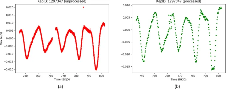
In Figure 1, we display an example light-curve quarter before and after preprocessing has been performed, respectively.
Finally, we concatenate all processed quarters of a single object into one large curve. To properly format the data for both the RNN and feature engineering approaches, all curves must be the same length; therefore wefind the longest resulting light curve and prepend all others with−999s until they are the same length. The−999 value is distinct and is masked out later in the training and testing process.
This process reduced the initial 234,000 quarterfiles down to just over 48,500 unique object light curves, each with a length of∼7000 time slices.
4
https://mast.stsci.edu
5
https://archive.stsci.edu/kepler/catalogs.html
6
2.2. Labels
The stellar properties used as labels in the classification and regression tasks were extracted from theKeplerStellar 17 table on MAST.7 This table includes properties for more than 200,000Keplertargets, and of the 95 columns describing each target,8we use the 10 properties given in Table 1to generate labels for 10 distinct prediction tasks.
3. Method
As stated in the introduction, we approach the problem of extracting and identifying physical properties of the star through two methods: representation learning, and feature engineering. In the sections below, we describe how each method was implemented. Results and discussion for each approach follow in subsequent sections.
3.1. Machine Learning Introduction
Machine learning attempts to automate the data analysis process. Much of this is done by exploiting the tools of
probability theory. There are many differentflavors of machine learning, but it is usually divided into two main types. In predictive or supervised learning, the goal is to learn a mapping from inputs to outputs given a labeled set of input-output pairs (the training set). The second main type is descriptive or unsupervised learning, where we are only given inputs and the goal is tofind interesting patterns in the data. Within this space, one can perform either classification(pattern recognition)when the problem is categorical, or regression tofind a specific value (Murphy 2012). There are a large variety of algorithm approaches to machine learning. These include (as a few examples) Bayesian, clustering, ensemble, instance based, ANNs, regularization, and feature engineering.
ANNs are a much-lauded tool of machine learning, popular for their flexibility and power. ANNs can be thought of mathematically as a form of function approximation and are used for tasks such as regression and classification. ANNs have a large number of tunable parameters, all of which fall into two categories. The weights and biases are internal parameters, selected via an optimization routine (e.g., stochastic gradient descent) over a chosen metric (e.g., mean squared error; Bottou2010). The hyperparameters include width, which is the number of nodes per layer, and depth, which is the number of layers stacked to form the network. Increasing the depth leads
Figure 1.Demonstration of before(a)and after(b)light-curve preprocessing on a single quarter. Table 1
Ten Stellar Properties Used to Generate Labels for Corresponding Object Light Curves in Prediction Tasks
Parameter Name Description Units Minimum Maximum Prediction Task
teff Effective Temperature K 2500 27730 Regression
logg Surface Gravity log10(cm s−2) 0.016 5.52 Regression
feh Metallicity dex −2.5 1 Regression
mass Mass Me 0.09 3.74 Regression
radius Radius Re 0.104 300.749 Regression
dens Density g cm−3 0 124 Regression
kepmag Kepler-band Magnitude mag −0.419 17.394 Regression
nconfp Number of confirmed Planets L 0 7 Classification
nkoi Number of Associated KOIsa L 0 7 Classification
ntce Number of Associated TCEsb L 0 8 Classification
Notes.
a
Keplerobjects of interest.
b
Threshold crossing events, e.g., exoplanet transits.
7
Found at:https://archive.stsci.edu/pub/kepler/catalogs/.
8
Parameter information further discussed athttp://archive.stsci.edu/kepler/ stellar17/help/columns.html.
to deep learning, where the definition of deep learning tends to change with advances in computation. In general, increasing depth and width enables better performance, where depth is thought to have a greater payoff. Note that as depth and width increase, so does computation time.
Every ANN consists of nodes and edges, with an example ANN shown in Figure 2. The nodes of the input layer correspond to the input data; the number of input nodes corresponds to the dimensionality of that data. For example, if we are interested in 8×8 pixel grayscale images, the number of input nodes will be 64. The nodes of the output layer depend on the task for which the ANN was designed. If the network was designed to predict a single number, then there will be a single output node. If the intent is to classify an input image among k categories, one would choose k output nodes, each corresponding to the probability that the input data belong to a particular category. The nodes of the hidden layer correspond to intermediate data transformations, which are governed by both the learned weights and biases, and the hyperparameters. The arrows in Figure2denote theflow of data between nodes; the example is a densely connected feed-forward network, where data are allowed to flow between all nodes (densely connected), but only in one direction (feed-forward).
The details of each individual node are shown in Figure2in the diagram on the right. Each node takes some number of inputs, combines them, feeds them through an activation function, and the result is then passed on to some other number of nodes. The combination of inputs is usually scaled by individual weights, then added along with a bias term. The weights and biases are chosen via optimization, but the activation function is chosen a priori. The choice of activation function is a topic of active research, but a current popular choice is the rectifier(Glorot et al. 2011).
There are several flavors of ANNs, but two of the most popular are RNNs and CNNs. An RNN is an ANN with internal memory. What this means is that information is allowed to pass between nodes in the same layer. If both forward and backward propagation are allowed, then the RNN becomes bi-directional. A popular form of RNNs is the LSTM RNN, which provides facilities for memory management, including the ability to forget or reset an internal state (Sak et al.2014). A CNN is an ANN that assumes some invariance structure of the input data, and therefore enforces invariance in
the structure of the ANN(Zhang et al.1990). The network is invariant in the sense that it applies the same small set of weights and biases to different portions of the input data. More specifically, the network performs convolution of learned kernels against the input data. This design choice reduces the number of internal parameters, decreasing the expense of training. Convolving against a kernel can be thought of as searching for patterns. Mishkin et al. (2016) details an investigation of different CNN design choices and their relative performance.
A more thorough discussion about machine learning in general can be found in Murphy(2012), and neural networks in particular are discussed in the review article by Schmidhu-ber(2015).
3.2. Representation Learning
In an effort to understand which properties we can obtain from stellar light curves, we turn to representation learning techniques. Representation learning allows the model to extract the “features” that it finds to be important in characterizing objects according to one physical property at a time. While this may initially limit model interpretability, it provides an opportunity for hidden features of the light curve to surface and help in classifying an object by various stellar properties. While feature engineering can be extensive, representation learning has the opportunity to remove human-based pre-conceived notions about what may or may not affect a starʼs classification.
In line with more common natural language processing tasks, we treat each set of 48,500 light curves as a corpus, with each light curve simulating a sentence and each normalizedflux measurement simulating a word. By implementing an LSTM RNN, we hope that the model will learn both semantic relations betweenflux values in a sequence and the more general pattern meanings throughout the “corpus” of objects, allowing the model to make accurate stellar predictions. A similar approach of treating a light curve as a sentence was done by Charnock & Moss(2017)in their analysis of supernovae light curves.
3.2.1. Network Architecture
We referred to related literature when determining the model architecture—primarily Charnock & Moss (2017), which
Figure 2.Left: Schematic for a simple artificial neural network with a depth of two and unspecified width. Right: Schematic for a simple, generic node. Here three inputsxiare scaled by weightswi, summed, and biased b before being fed through an activation functionf(y).
optimized an LSTM RNN in classifying supernovae light curves. In addition to similar data structures, Charnock & Moss had a comparable data set size (although simulated) and analogous prediction tasks, leading us to use a similar model structure and complexity. Our LSTM RNN was built in python using the Keras neural network library.9The ideal architecture was found to be an RNN with two LSTM hidden layers of 16 nodes each(and an initial masking layer tofilter out prepended
−999s), although we initially ran tests on just a single hidden layer to reduce computation time. An example of a generic RNN with two LSTM hidden layers can be seen in Figure3.
In building the LSTM RNN, we wished to perform two types of predictive tasks: binary classification(does an object belong to one class or another?), and regression (what is the numerical value of this star’s physical property?). For both LSTM layers we used a softmax activation function for classification tasks and a softsign activation function for regression tasks. The dense layer was always assigned a linear activation function. In network compilation, a categorical cross-entropy loss was used for classification tasks and a mean squared error loss for regression tasks. We applied the RMSProp10optimizer with default learning rate. Whenfitting, a batch size of 20 was used and in both classification and regression tasks, and we surveyed the reported loss values between epochs to determine when performance had plateaued (namely, when loss values seemed to converge). Weights were balanced using scikit-learnʼs class_weight utility function specifying“balanced”weights. This process effectively returns the frequency of each class, or more specifically, each class weight=(number of samples)/(number of classes∗number of samples belonging to that class). Once a list of class weights were obtained, we fed the list into the neural network when fitting. All other parameters not specified here were Keras layer defaults. More specifics on these modifications for the two tasks are discussed below.
3.2.2. Modifications
We decided to perform classification tasks on the parameters with discrete values within a limited set (i.e., number of confirmed planets, number of associated Kepler objects of interest (KOIs), and number of associated threshold crossing events(TCEs)). However, while the sets of possible values for each of these properties are already quite limited, each of these three parameters is heavily dominated by negative signals(i.e., a value of zero). Thus, we decided to simplify the tasks further by making each binary classification task either equal to or greater than zero. However, despite the classification simpli-fication, the data still consisted of a skewed population for each of the three relevant properties. To combat heavy bias, we instantiated the model with balanced weights, such that the model would weight the importance of positive labels more highly than negative labels to avoid converging as a simple majority class predictor.
The key to creating a classification model versus a model that performs regression tasks is primarily in the structure of the output layer. We implemented one node for each class of the classification task (two for binary classification)in the output layer. Additionally, the loss function(a metric over which each model is optimized)varies slightly between classification and regression tasks. Since we wish to correctly categorize the target, we apply a categorical cross-entropy loss function, provided below:
å
= - ( ) Li t log p . j i j, i j,The loss function is applied to each prediction targetiand each of thejpossible classes(e.g.,j=2 in our binary predictions), wheretis the target or actual probability that an object belongs to that class, andp is the corresponding predicted probability. This function is minimized by the neural network to optimize prediction tasks.
Rather than creating multiple nodes in the output layer as was done for the classification tasks, regression tasks require just a single node. This means that the output will be the estimated property value, rather than a set of weights
Figure 3.Example of the data and label inputs and architecture of a recurrent neural network with LSTM nodes to predict and classify stellar properties.
9
The Keras deep learning library is an open source library developed by Francois Chollet at the MIT in 2015. More information can be found athttps://keras.io/.
10
corresponding to the modelʼs confidence in each respective class.
3.2.3. Evaluation Metrics
In determining the success of a predictive model, various evaluation metrics are used to measure results. These are not used in the training process, but are helpful when considering how well the model performed on a certain task. The metrics come from entries in a confusion matrix (Kohavi & Provost 1998)that contains information about the actual and predicted classifications done by a classification system. Performance of the system, in our case, our machine learning methods, is evaluated using the data contained in the confusion matrix.
For a binary classifier we utse a two-class matrix, also known as a truth table, as seen in Table 2.
Traditional or“raw”accuracy is simply defined as the ratio between the number of correct predictions and the total number of predictions. For two classes, raw accuracy is calculated as
=( + ) ( + )
Accuracy TP TN P N ,
where TP is the number of true positives, TN is the number of true negatives, P is the total number of positives, and N is the total number of negatives.
Therefore, a random binary classifier would have an accuracy of 1/2 and a random classifier with three classes would have an accuracy of 1/3. Each of our classification tasks contained extremely imbalanced data, where the number of “positive” samples (i.e., a confirmed transit) was lower than 10% of the total data set for each parameter. Therefore raw accuracy returned misleadingly high values even for a simple majority class predictor and was not an appropriate metric to evaluate prediction performance.
Therefore we turned to balanced accuracy using a confusion matrix of predictions. For binary classification problems, the confusion matrix splits predictions into true positives (TP), false positives (FP), false negatives (FNs), and true negatives (TNs). Balanced accuracy is then defined as
=( + )
Balanced Accuracy TP P TN N 2.
Additionally we can calculate the recall of a model, which tells us how many positive cases were correctly identified, and the precision, which tells us how many of those predicted positive cases were correctly identified. Recall is defined as
= ( + )
Recall TP TP FN ,
and precision is defined as
= ( + )
Precision TP TP FP .
From recall and precision, we can calculate theF1score, which
can be used to measure the accuracy of the model. It uses both recall and precision (which are obtained from the truth table). TheF1score provides a harmonic average of the precision and
recall, where the best value forF1is 1 and the worst is 0.F1is described as = * * + F 2 Precision Recall Precision Recall. 1
3.2.4. Representation Learning(LSTM RNN)Results
We found that both the classification and regression results resulted in approximately guessing accuracy. For classification, the balanced accuracy was approximately 52% for all three tasks, and for regression, the RNN was onlyfinding the average of all of the values instead of predicting the individual value. Previous successful work had centered on simulated data (Charnock & Moss) or other types of representation learning (self-organizing map (SOM) in the case of Armstrong et al. (2017))and it is possible that the variation in the light-curve data, the relatively small sample set of 48,500 light curves, or the ratio of positive samples to negative was too low for the RNN to predict values.
Upon these results, we were driven to explore another machine learning method with more human knowledge in the loop—namely feature engineering.
3.3. Feature Engineering
To attempt to improve our ability to perform prediction tasks, we turned to feature extraction to construct feature representations of the light curves. This strategy is commonly referred to as feature engineering. Feature engineering is the process of determining, calculating, and extracting features from raw data. These features are typically properties of the raw data that are human interpretable and believed to provide insight on the prediction task at hand. While this process can be arduous(feature engineering often takes quite long and may be computationally intensive), it also provides useful intuition into our understanding of certain properties and patterns of the raw data. Furthermore, the fact that feature engineering typically uses human-crafted properties allows us to perform a more in-depth data analysis on why certain features predict certain physical properties. While representation learning is able to extract“features”from raw data for unexpected insight, it does not offer the depth of insight that feature engineering can provide.
In order to extract features from light curves, we turned to FATS, the feature analysis of time series (Nun et al. 2015). Since there is extensive documentation for FATS on its Github repository11 and within Nun et al. (2015), here we only summarize how we extracted features from our preprocessed light curves. FATS takes time-series data, and depending on the target, extracts mathematical properties and statistical information(Nun et al.2015). While FATS can be applied to a variety of time-series data, we focus on using it to extract features from light curves. Specifically, we extract 46 features from 6038 light curves and train them on the following models: naïve Bayesian, K-nearest neighbors, support vector machine, decision tree, random forest, L1-norm regression, L2-norm
Table 2
Truth Table where TN is the Number of True Negatives, FN is the Number False Negatives, FP is the Number of False Positives, and TP is the Number of
True Positives
Predicted Value Actual Value
0 1
0 TN FN
1 FP TP
Note.These values are used in calculating the metrics used to evaluate model performance.
11
regression, and support vector regression(SVR). This analysis was performed on the same data prepared in the LSTM RNN experiment. Hyperparameters were determined by a simple script that trained from 1 to N classifiers and chose the value that minimized out of sample error. The main data set was split into a testing and training set such that the training set was 80% of the data and the testing set was 20% of the data. Each model used for classification utilized a function to calculate out of sample error, and each model used for regression utilized a function that provided RMSE as an output.
3.3.1. Feature Selection and Extraction
To accurately simulate the type of information we will be receiving from future synoptic surveys, we use only magnitude and time measurements from the light curve as inputs to FATS. Given magnitude and time, there are a total of 53 features that can be calculated. Out of these 53, we exclude 7 features. FluxPercentileRatioMid20, FluxPercentileRatioMid35, PercentileRatioMid50, FluxPercentileRatioMid65, and Flux-PercentileRatioMid80 were excluded because they produce values of infinity during feature generation. This issue is a product of the preprocessing done on the light curves, which centered each time series around 0. FluxPercentileRatio*was calculated using the formula
*=F *
F FluxPercentileRatio 50 2,
5,95
whereF5,95is the difference between 95% and 5% of theflux. This difference was occasionally truncated to zero by Python if it was too small. This led to values of infinity that were removed from the list of features as they do not provide reliable information. We also discarded percent amplitude and percent differenceflux percentile. Percent amplitude is calculated as
= ⎛ ⎝ ⎜ ⎞ ⎠ ⎟ F F F F Percent Amplitude max min ,
median max median and percent difference flux percentile from
= F
F Percent Difference Flux Percentile 5,95 .
median
Both of these values rely on the median flux value, which on occasion is equal to zero as the data were normalized to be centered around zero. Again, during feature generation, some of the light curves held values of infinity for these two properties, and so we discarded them with the same reasoning as for the FluxPercentileRatio*values. Therefore we were left with 46 features, which are listed in Table3.
3.3.2. Feature Engineering Regression Results
We ran three different regression models to predict values for stellar surface gravity(log(g)), stellar mass(in units ofMe), density, stellar radius(in units ofRe), and the stellar effective temperature. Thefirst two models are linear regression models. The benefits of linear regression is its simplicity in both implementation and interpretability. Its drawback comes when the relationship between the inputs and outputs cannot be approximated by a linear relationship, in which case the model will give poor predictions. The two linear methods we used are the least absolute shrinkage and selection operator (LASSO; Tibshirani 1996) and ridge regression (Rasmussen &
Williams 2006), which we have denoted L1 regression and L2 regression, respectively. L1 regression is“robust”, meaning that it does not overlyfit to outliers, it is“unstable”such that small adjustments in the data have the potential to move the regression fit, and it has multiple solutions. L2 regression is “not robust”, so it could have a tendency to overfit; it is stable, so the regression line is not affected by small data adjustments; and it has a unique solution.
The third method is a nonlinear method called SVR. It was originally developed for classification problems and later extended to regression. It is useful when the relationship between the inputs and outputs are not best fit by a linear relationship. For a full description of the methods, we refer to Rasmussen & Williams(2006)and Murphy(2012). The results obtained for regression are described in terms of root mean squared error(RMSE)and are shown in Table4. We recall that RMSE is calculated within each of the regression models.
Where the range in values for each stellar property is listed in Table5.
To enable a better comparison for the performance of each model in predicting these values, we then normalized the RMSE, which can be seen in Table6.
Feature engineering for regression proved to give good predictions for stellar surface gravity and stellar mass, and very good predictions for stellar density, stellar radius, and effective stellar temperature with both of the linear models performing slightly better than SVR. SVR is only better for predicting the stellar mass and is pretty even with the linear models for predicting stellar surface gravity, but overall, the differences between the models are minor. This technique could be used with confidence to classify the large database of unclassified stars without immediate need for follow-up observations.
3.3.3. Feature Engineering Classification Results
Classification was performed on three separate types of events: number of TCEs, number of confirmed planets, and number of KOIs.
3.3.3.1. Feature Importance
Using FATS for each of these classification events, we calculated the importance of each of the features from Table3. Ourfirst look was the number of KOIs in a given light curve. As we see in Figure 4, mean, skew, and freq1HarmonicsRel. Phase1 are all features that contribute greatly to understanding if an object of interest is contained within the light curve for a model using a random forest classifier.
Figure 5 shows the relative feature importance for the number of TCEs. Here different features, namely the Period Lomb–Scargle and Etae, are the two most dominant features,
but the freqN HarmonicsRel.Phase terms are not important at all to the classification.
Finally, Figure 6 shows the relative feature importance for the number of confirmed planets. Here we see that the freq1_harmonics_rel_phase_1 is the dominant feature followed by skew, with the features not contributing to the classification being the different freq_harmonics_rel_phase0 terms. This analysis shows us that even for seemingly fairly related events, the feature importance can vary greatly when it comes to classification.
Table 3
Features Generated from FATS Used in Machine Learning Methods
Feature Input Data(in addition to magnitude) Parameters Default Reference
Amplitude L L L Richards et al.(2011)
AndersonDarling test L L L Kim et al.(2009)
Autocor length L Number of lags 100 Kim et al.(2011)
Con L Consecutive Stars 3 Kim et al.(2011)
Etae Time L L Kim et al.(2014)
Freq1HarmonicsAmp0 Time L L Richards et al.(2011)
Freq1HarmonicsAmpi Time L L Richards et al.(2011)
Freq1HarmonicsRelPhase0 Time L L Richards et al.(2011)
Freq1HarmonicsRelPhasei Time L L Richards et al.(2011)
Freq2HarmonicsAmp0 Time L L Richards et al.(2011)
Freq2HarmonicsAmpi Time L L Richards et al.(2011)
Freq2HarmonicsRelPhase0 Time L L Richards et al.(2011)
Freq2HarmonicsRelPhasei Time L L Richards et al.(2011)
Freq3HarmonicsAmp0 Time L L Richards et al.(2011)
Freq3HarmonicsAmpi Time L L Richards et al.(2011)
Freq3HarmonicsRelPhase0 Time L L Richards et al.(2011)
Freq3HarmonicsRelPhasei Time L L Richards et al.(2011)
Linear Trend Time L L Richards et al.(2011)
Max Slope Time L L Richards et al.(2011)
Mean L L L Kim et al.(2014)
Mean Variance L L L Kim et al.(2011)
Mean Absolute Deviation L L L Richards et al.(2011)
Median BRP L L L Richards et al.(2011)
PairSlopeTrend L L L Richards et al.(2011)
Period Lomb–Scargle Time Oversampling Factor 6 Kim et al.(2011)
Period Fit Time L L Kim et al.(2011)
ψcs Time L L Kim et al.(2014)
ψη Time L L Kim et al.(2014)
-Q3 1 L L L Kim et al.(2014)
RCS L L L Kim et al.(2011)
Skew L L L Richards et al.(2011)
Slotted AutoCor Length Time Slot Size T(days) 4 Protopapas et al.(2015)
Small Kurtosis L L L Richards et al.(2011)
Standard Deviation L L L Richards et al.(2011)
Note.In the“freqN Harmonics”Terms,i=1–3.
Table 4
Feature Engineering Results for Regression Root Mean Squared Error
Model Stellar Surface Gravity(log(g)) Stellar Mass(Me) Density(g cm−3) Stellar Radius(Re) Effective Temperature(K)
L1 ±0.9088 ±0.6604 ±2.699 ±14.26 ±879.6
L2 ±0.8254 ±0.6341 ±2.669 ±13.25 ±875.4
SVR ±0.8735 ±0.6050 ±2.829 ±19.87 ±967.2
Table 5
Range of Values for Each Stellar Property
Stellar Surface Gravity(log(g)) Stellar Mass(Me) Density(g cm−3) Stellar Radius(Re) Effective Temperature(K)
Range 0.016–5.52 0.09–3.74 0–124 0.104–300.749 2500–27730
Table 6
Normalized RMSE for Each of the Stellar Properties with Each Different Model Normalized Root Mean Squared Error(%)
Model Stellar Surface Gravity(log(g)) Stellar Mass(Me) Density(g cm−3) Stellar Radius(Re) Effective Temperature(K)
L1 ±0.1651 ±0.1809 ±0.0217 ±0.0474 ±0.0348
L2 ±0.1499 ±0.1737 ±0.0215 ±0.0441 ±0.0347
Using these results, we can reduce the data to only the features that hold importance for the classification tasks at hand and improve the overall classification accuracy.
3.3.3.2. Classification Results
Upon running each of thefive classifier models, we are able to see how well each type predicts the correct value based on
the two metrics: out of sample error(Eout), which measures the
difference between the expected and empirical error, and balanced accuracy. To calculateEout, wefirst used the training
data on the scikit learn model. After it was trained, we used it to predict the classes of the testing data. Since the classes of the testing data are known, we can compare them to the class that the model predicts. We predicted all of the classes for each data
Figure 4.Feature importance in random forest NKOI classification.
point in the testing data and for every data point misclassified, we incremented a counter. After each pointʼs class was predicted, we divided the total number of points in the testing data to obtain the ratio of points that were misclassified. The calculation for balanced accuracy can be seen in Section3.2.3. Our experiment was to check if the machine learning method could pull from a complete set of noisy/sparseKeplerdata the correct values for each of the classifications described below. For the number of KOIs, we had the model classify whether a given star had at least one KOI associated with it. The performance of each of the models for KOI is in Table 7.
Here we see that a naïve Bayesian model has a very highEout
and guessing-level balanced accuracy. Each of the others have a small out-of-sample error, and the model appears to be moving beyond simply guessing. These values of balanced accuracy are promising.
Turning to the number of TCEs in Table 8, we start to see more favorable values for balanced accuracy. Here the models were ran against the full light-curve set to determine if a given star had a transit event.
Here, again, we see that a naïve Bayesian model is not a good classifier for determining the number of TCEs. It has a large out-of-sample error, and its balanced accuracy is that of guessing. Each of the other model types are better to varying degrees. Decision trees produced the best balanced accuracy, but had a slightly higher out-of-sample error than that of a random forest of 1000 trees, which produced the least out-of-sample error and a very respectable value for balanced accuracy. When compared to other examples using noisy sparse data with multi-layer neural networks in the extended physics community, the model is classifying fairly well. As an example in a related field where the signal of interest (Higgs boson)is an extreme minority in the an otherwise large data set, the use of deep neural networks for classifying the Higgs boson
at the LHC (Alves et al. 2017) achieved accuracies ranging from(∼60%–84%).
Finally, we look at the number of confirmed planets per stellar light curve in Table9. Here we wished to see if we could move beyond a potential transit and determine if the method could identify planets with some degree of confidence. This would be very attractive as it would allow a set of data to be evaluated against training data containing confirmed planets and confidently tell us that a star that has yet to be analyzed indeed has a planet.
Figure 6.Feature importance in random forest number of threshold crossing events classification.
Table 7
Comparison of Classifier Models for Classifying the Number ofKeplerObjects of Interest for a Given Set of Light Curves
Number ofKeplerObjects of Interest
Classifier Eout(%) Balanced Accuracy(%)
Naïve Bayes 92.38 51.15
SVM 5.71 57.72
KNN 4.72 58.96
D-Tree 8.19 62.82
Random Forest(1000 Trees) 4.64 57.58
Table 8
Comparison of Classifier Models for Classifying the Number of Threshold Crossing Events for a Given Set of Light Curves
Number of Threshold Crossing Events
Classifier Eout(%) Balanced Accuracy(%)
Naïve Bayes 87.25 50.04
SVM 14.98 66.86
KNN 10.84 62.77
D-Tree 13.99 71.53
This classification proved to be difficult for all five classifiers. Here SVM, KNN, and random forests were all guessing a classification of zero(i.e., no confirmed planets). It only makes sense that the model might revert to this since the sample size is very small for light curves containing confirmed planets and even smaller for light curves with multiple planets.
3.3.4. Further Analysis
After achieving thefirst set of results, we decided to define what might be causing such low model performance. We determined that our classification problems are heavily imbalanced, where the minority class (such as a light curve with a confirmed planet) is significantly smaller than the majority class(light curves without confirmed planets). To help remedy this, we turned to a method to attempt to oversample the minority class. Specifically, we used the synthetic minority oversampling technique, or SMOTE (Chawla et al.2002).
In many cases with real data, the interesting examples within the data can be severely underrepresented, making classifi ca-tion difficult. The machine learning community has approached this probably through both resampling the original data set (either by oversampling the minority class or undersampling the majority class; Lewis & Catlett 1994; Kubat & Matwin1997; Ling & Li1998; Japkowicz2000)or by adding costs to the training examples (Pazzani et al. 1994; Dom-ingos1999). SMOTE provides an approach that combines both oversampling the minority (or interesting) class and under-sampling the majority class. Chawla et al.(2002)used several different classifiers(C4.5 decision trees; Quinlan 1992; naïve Bayes, and ripper; Cohen 1995b) and showed that this combined method achieves better performance.
This algorithm does the following:
(1)Takes the minority class sample, xi, and its k minority class nearest neighborsy1....yk.
(2)Introduces n synthetic examples along the line segments joining xiwith itskneighbors.
(a)Take the difference between yjand xi.
(b)Multiply the difference by number between zero and one.
(c)Add the difference to xi.
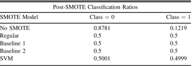
We chose to apply this to our most promising classification set, the number of TCEs. Table 10 shows our post-SMOTE classification ratios, where class=0 represents light curves without a crossing event, and class=1 where a crossing event is detected.
As one can see, the data are dominated by class=0 events, but by applying the various versions of a SMOTE model, we achieve closer to a 50/50 ratio of class=0 and class=1
events. To provide additional metrics for model performance with the addition of SMOTE, we calculated recall and precision. Recall is defined as
= ( + )
Recall TP TP FN ,
which is basically the ratio of positives that are correct out of all actual positives, and precision is defined as
= ( + )
Precision TP TP FP ,
which is the ratio of positives that are correct out of all guessed positives.
Table11 shows the previously reported Eout and balanced
accuracies as well as recall and precision for each model classifier.
After applying SMOTE to our data, we saw that the SMOTE SVM achieved the greatest improvement in results, which can be seen in Table12.
Table 9
Comparison of Classifier Models for Classifying the Number of Confirmed Planets for a Given Set of Light Curves
Number of Confirmed Planets
Classifier Eout(%) Balanced Accuracy(%)
Naïve Bayes 94.54 52.23
SVM 0.745 55
KNN 0.745 55
D-Tree 1.49 54.62
Random Forest(1000 Trees) .745 55
Table 10
Model Results Before and After Applying SMOTE to Balance the Majority/ Minority Class
Post-SMOTE Classification Ratios
SMOTE Model Class=0 Class=1
No SMOTE 0.8781 0.1219 Regular 0.5 0.5 Baseline 1 0.5 0.5 Baseline 2 0.5 0.5 SVM 0.5001 0.4999 Table 11
Comparison of the Classifier Models Including Recall and Precision as Metrics Number of Threshold Crossing Events(NCTE)
Classifier Eout(%)
Balanced Accuracy
(%) Recall Precision F1Score
Naïve Bayes 87.25 50.04 0.993 0.122 0.217 SVM 14.98 66.86 0.429 0.394 0.411 KNN 10.84 62.77 0.279 0.621 0.385 D-Tree 13.99 71.53 0.517 0.409 0.457 Random For-est(1000 Trees) 8.029 69.94 0.395 0.828 0.535 Table 12
Comparison of the Classifier Models After Applying SMOTE to the Minority Class
NTCE with SMOTE SVM
Classifier Eout(%)
Balanced Accuracy
(%) Recall Precision F1Score
Naïve Bayes 85.4 50.5 0.980 0.123 0.219 SVM 13.2 65.8 0.381 0.452 0.413 KNN 21.4 62.0 0.517 0.289 0.371 D-Tree 17.1 69.8 0.524 0.362 0.428 Random For-est(1000 Trees) 8.86 74.7 0.530 0.672 0.593
Note.Note the improvement in balanced accuracy for the random forest and the trade-off for achieving better recall at the sacrifice of some precision.
The naïve Bayesian model still produced guessing results with a high Eout. However, the use of SMOTE greatly
improved the random forest, in particular, achieving almost 75% balanced accuracy. Additionally, in all cases but the D-tree, the F1 score slightly improved. As a comparison, Armstrong et al.(2017)achieved a 87% accuracy with an SOM neural network for finding the true planet detections and discarding the FPs among the KOIs. While the methods used in Armstrong et al. (2017) and our work are very different, the results give us an idea about the type of accuracy that is obtainable with realKepler data.
With more data containing positive detections and additional data conditioning, a SMOTE feature engineering method could be useful in achieving insight into exoplanet presence in a given stellar system. This could provide astronomers a useful tool for quickly identifying stellar systems with an extremely high likelihood of exoplanet presence, allowing for more focused analyses.
4. Discussion
While the results from the LSTM RNN were initially disappointing, this led us to investigate feature engineering for both regression and classification problems. Feature engineer-ing provided excellent results for regression and very promising results for classification. Once we achieved some confidence in the approach, we decided to employ the SMOTE technique on our data set to remove the severe imbalance. After employing SMOTE, the classification results greatly improved. The classification balance accuracy is in line with other results with real data (using different methods), but still does not achieve the ∼90%–95% that is achieved with simulated data (Charnock & Moss2017). Noisiness and sparseness of the data appear to play a large role in the ability to classify real light-curve data with machine learning techniques, but improve-ments in performance can be made using minority class oversampling techniques such as SMOTE.
Initially, we thought that the poor results from the LSTM RNN were entirely due to the noisiness and sparseness of the data and that light curves may not be suited to analysis with an RNN. However, with the success of SMOTE, we now think that there may be techniques to boost the minority class and potentially improve the performance of representation learning methods with real astrophysical data. It should be noted that SMOTE cannot be used on time-series data as it is dependent upon existing in feature space and is not applied to raw time-series data. Future work will be to investigate such methods and test if the LSTM RNN can be more successful with data augmentation. This reinvestigation could be complementary to the work by Naul et al. (2018)using RNN feature extraction.
The success of the feature engineering approach(particularly with stellar property prediction)gives us confidence that these techniques will make useful tools for the astronomy community when beginning to analyze the large volume of data that will be available with TESS and theJWSTand provide better guidance in using precious revisit time from ground-based observatories.
5. Summary
With the eminent boom of astronomical data on the horizon, new methods and techniques need to be developed and refined to reduce analysis time, increase accuracy, and provide new insights into the data themselves. We attempt to add techniques
to the community through investigating representation learning and feature engineering approaches to better understand what may be possible.
Upon investigation, we discovered that our LSTM RNN approach to representation learning was limited in its applicability. This was either due to the limited positive sample size within our data or the sparseness and/or noisiness of real data, since successful applications of RNNs have been shown primarily on simulated data where noise is also simulated and therefore more predictable.
While representation learning did not prove to be ideal, feature engineering provided excellent results with regard to both regression and classification. For regression, the model could predict values for density, stellar radius, and effective temperature, where the ridge regression model performed the best with a normalized RMSE of±0.0215,±0.0441, and±0.0347 for each value, respectively. Classification results showed that a random forest of 1000 trees produced the lowest out-of-sample error at 8.86% with a balanced accuracy of 74.7%. Upon inspection of the literature in the community, this may be the first comparative study of machine learning methods using real astronomical data. We hope that this work will be informative and provide a base for future endeavors both from our team and the extended community.
We would like to thank theKeplerteam for making all of the data publicly available on MAST. We would also like to thank Sara Seager (MIT) and David Hogg (NYU) for discussions, encouragement, and advice. This work was supported by Northrop Grumman Corporation.
References
Alves, A., Ghosh, T., & Sinha, K. 2017,PhRvD,96, 035022
Armstrong, D. J., Pollacco, D., & Santerne, A. 2017,MNRAS,465, 2634 Bailey, S., Aragon, C., Romano, R., et al. 2007,ApJ,665, 1246 Ball, N. M., & Brunner, R. J. 2010,IJMPD,19, 1049
Bastien, F., Stassun, K., Basri, G., & Pepper, J. 2015,ApJ,818, 43 Beichman, C., Benneke, B., Knutson, K., et al. 2014,PASP,126, 1134 Bottou, L. 2010, in Proc. COMPSTAT’2010, 177
Cabrera-Vives, G., Reyes, I., Forster, F., Estevez, P., & Maureira, J. C. 2017,
ApJ,836, 97
Charnock, T., & Moss, A. 2017,ApJL,837, L28
Chawla, N., Bowyer, K., Hall, L., & Kegelmeyer, W. 2002, Journal of Artificial Intelligence, 16, 321
Cohen, W. W. 1995b, in Proc. 12th Int. Conf. on Machine Learning, 115 Domingos, P. 1999, in Proc. Fifth ACM SIGKDD Int. Conf. on Knowledge
Discovery and Data Mining, 155
Glorot, X., Bordes, A., & Bengio, Y. 2011, in Proc. Fourteenth Int. Conf. on Artificial Intelligence and Statistics, 315
Japkowicz, N. 2000, in Proc. 2000 Int. Conf. on Artificial Intelligence Special Track on Inductive Learning
Karpenka, N. V., Feroz, F., & Hobson, M. P. 2013,MNRAS,429, 1278 Kim, D.-W., Protopapas, C., Byun, Y.-I., et al. 2011,ApJ,735, 68
Kim, D.-W., Protopapas, P., Alcock, C., Byun, Y.-I., & Bianco, F. 2009,
MNRAS,397, 558
Kim, D.-W., Protopapas, P., Bailer-Jones, C. A. L., et al. 2014, A&A, 566, A43
Kohavi, R., & Provost, F. 1998, Editorial for the Special Issue on Applications of Machine Learning and the Knowledge Discovery Process, Vol. 30(New York: Columbia Univ.)
Kubat, M., & Matwin, S. 1997, in Proc. Fourteenth International Conf. on Machine Learning, 179
Lewis, D., & Catlett, J. 1994, in Proc. Eleventh Int. Conf. of Machine Learning, 148
Ling, C., & Li, C. 1998, in Proc. Fourth Int. Conf. on Knowledge Discovery and Data Mining(KDD-98)
Murphy, K. P. 2012, Machine Learning: A Probabilistic Perspective
(Cambridge, MA: MIT Press)
Naul, B., Bloom, J. S., Perez, F., & van der Walt, S. 2018,NatAs,2, 151 Nun, I., Protopapas, P., Sim, B., et al. 2015, arXiv:1510.05988
Pazzani, M., Merz, C., Murphy, P., et al. 1994, in Proc. Eleventh Int. Conf. on Machine Learning
Protopapas, P., Huijse, P., Estévez, P. A., et al. 2015,ApJS,216, 25 Quinlan, J. 1992, Programs for Machine Learning(Burlington, MA: Morgan
Kaufmann)
Rasmussen, C. E., & Williams, C. K. I. 2006, Gaussian Processes for Machine Learning(Cambridge, MA: MIT Press)
Richards, J. W., Starr, D. L., Butler, N. R., et al. 2011,ApJ,733, 10 Sak, H., Senior, A., & Beaufays, F. 2014, in Fifteenth Annual Conf. Int.
Speech Communication Association Schmidhuber, J. 2015,NN, 61, 85
Spencer, R. 2013, in IET Seminar on Data Analytics 2013: Deriving Intelligence and Value from Big Data
Thompson, S., Mulally, F., Coughlin, J., et al. 2015,ApJ,812, 46
Tibshirani, R. 1996, Journal of the Royal Statistical Society. Series B, 58, 267 Wang, D., Hogg, D. W., Foreman-Mackey, D., & Scholkopf, B. 2016,
arXiv:1508.01853v2