Missing values imputation and image registration for genetics applications

(1)

c

(2)

MISSING VALUES IMPUTATION AND IMAGE REGISTRATION FOR GENETICS APPLICATIONS

BY

REBECCA CHEN

THESIS

Submitted in partial fulfillment of the requirements

for the degree of Master of Science in Electrical and Computer Engineering in the Graduate College of the

University of Illinois at Urbana-Champaign, 2019

Urbana, Illinois Adviser:

(3)

ABSTRACT

In this thesis, we address several common scenarios of corrupted data in data and image processing pipelines. The first is in the setting of clustered data with missing values. We design an algorithm for imputing missing values using optimal recovery and derive an error bound for non-negative matrix factorization of the imputed data. Second, we consider missing values as erasure channels and show examples of using Fano’s inequality to find lower bounds on missing values algorithms. Finally, we perform image registration of misaligned and noisy images using multiinformation and use finite rate of innovation sample to speed up registration while preserving optimality.

(4)

ACKNOWLEDGMENTS

I would like to thank my family, my husband, and my adviser for their support and guidance.

In addition, this work was supported in part by Air Force STTR Grant FA8650- 16-M-1819 and in part by grant number 2018-182794 from the Chan Zuckerberg Initiative DAF, an advised fund of the Silicon Valley Community Foundation.

(5)

CHAPTER 1

INTRODUCTION

Bioinformatics is an interdisciplinary field that has seen rapid growth in recent years due to the increased availability of biological data and advances in computer power. Modern technology has made it possible not only to store, but also to share large datasets. In addition, increases in computing power have made it possible to handle larger amounts of data than ever before. The goal is to extract useful information from the data that will allow us to understand biological systems.

The term “bioinformatics” was coined by Paulien Hogeweg and Ben Hesper in the 1970s to mean “the study of informatic processes in biotic systems” [1]. Hogeweg and Hesper proposed information storage, transmission, and processing as properties of living systems, and they considered this to be an important research area. This thinking was no doubt influenced by the devel-opment of the field of information theory in the 1950s and 60s, during which the Huffman code, the Reed-Solomon codes, and other landmark algorithms were developed. The idea that biological systems carried and transmitted in-formation was reflected in the coinage of the “genetic code” [1]. From within the field of theoretical biology emerged mathematical models of enzyme dy-namics and gene regulation. Alan Turing developed a theory for natural pattern formation (e.g. how a leopard gets its spots) [2]. Research in artifi-cial intelligence led to the development of genetic algorithms for optimization and the now-ubiquitous neural networks for pattern recognition.

The goal of bioinformatics soon evolved into one of data analysis and inter-pretation. This was due to a massive increase in public data brought about by advances in DNA sequencing techniques, including a rapid DNA sequenc-ing technique in 1977 and the polymerase chain reaction (PCR) technique for amplifying DNA in 1983. The U.S. Department of Energy (DOE) and the National Institutes of Health (NIH) set forth a plan to sequence the entire human genome, and in 1990, public funding for the Human Genome Project

(7)

(HGP) began. A parallel sequencing effort by Celera Genomics was formally launched in 1998. Celera developed a shotgun strategy that was able to sequence DNA more quickly and cost-effectively. This drove the HGP to improve their own technology, and both projects published their drafts of the completed human genome in 2000. The genome sequencing race spurred development not only in sequencing technology, but also in data mining, pattern recognition, and other analysis techniques.

Since then, technology has been developed for DNA methylation sequenc-ing, mRNA sequencsequenc-ing, and protein sequencsequenc-ing, allowing scientists to study genetic processes in a more nuanced way [3]. While every cell belonging to an individual contains the same set of DNA, the mRNA differ from cell to cell depending on the cell’s state and function (as do methylation and pro-tein expression). In 2016, an initiative called the Human Cell Atlas Project began. The project aims to create a comprehensive reference map of all the cells in the human body, with the goal of understanding human health and, ultimately, diagnosing and treating disease. Single-cell RNA sequenc-ing (scRNA-seq) has made it possible to capture gene expression patterns in individual cells. Beyond cell-level interactions, researchers hope to study tissue-level and eventually organ-level interactions, both spatially and func-tionally. Variations in gene expression patterns in healthy and diseased states can be compared, and temporal responses to drugs can be captured [4].

In this thesis we consider two facets of this genomics research: cell clus-tering and image-based transcriptomics. Clusclus-tering can be performed on gene-expression count matrices, which are matrices with cells on one axis and genes on the other axis. Matrix entries indicate the number of times a gene is expressed in a cell. Cells can then be clustered according to gene-expression patterns. Presumably, cells of different types or in different states will express genes differently. The second area we consider is image-based transcriptomics. Unlike gene counts, which only describe the abundance of genes in a cell, image-based transcriptomics captures spatial patterns of gene expression. In fluorescence in situ hybridization (FISH), genes are tagged by fluorescent markers, and images are taken in situ. Thus cellular microen-vironments, as well as localization patterns, are preserved. Single molecule FISH (sm-FISH) allows for single molecule sensitivity.

(8)

entirely. Low gene counts may be incorrectly recorded as zeros, but there is no easy way to determine whether a zero indicates the absence of a gene or a gene that was missed by the sequencing method. In chapter 2 we introduce patterns of missingness and describe methods of imputing, or filling in, miss-ing values. We cluster and impute data with missmiss-ing values usmiss-ing optimal recovery and find error bounds in the context of non-negative matrix factor-ization, which is a popular method for analyzing gene-expression matrices. In chapter 3 we discuss missing mechanisms as erasure channels and show an example of Fano’s inequality in a missing value setting.

In image-based transcriptomics, images must be aligned, or registered, so that the spatial configuration of the cell on the pixel grid matches across consecutive images. In chapter 4, we consider misaligned images as noisy copies of the original image and multivariate information functionals to per-form theoretically optimal registration. We then use finite-rate-of-innovation sampling to extract salient features, which speeds up registration while pre-serving optimality properties. Chapter 5 summarizes our findings and out-lines future work.

The basic approaches we develop are useful not just in bioinformatics but in other parts of data science and image processing also. Missing data is common in real-world settings, and image registration is used in hyperspec-tral remote sensing and many computer vision applications. Our methods can be readily applied to other applications.

Bibliographical Note

Part of Chapter 2 appears in

R. Chen, L. R. Varshney, “Non-negative matrix factorization of clustered data with missing values,” Proc. IEEE 2019 Data Sci. Workshop, 2019. Part of Chapter 4 appears in

R. Chen, A. B. Das, and L. R. Varshney, “Registration for image-based transcriptomics: Parametric signal features and multivariate information measures,” Proc. 53rd Conf. Inform. Sci. Syst., 2019.

(9)

CHAPTER 2

NON-NEGATIVE MATRIX

FACTORIZATION OF CLUSTERED DATA

WITH MISSING VALUES

2.1

Introduction

Matrix factorization is commonly used for clustering and dimensionality re-duction in computational biology, imaging, and other fields. Non-negative matrix factorization (NMF) is particularly favored by biologists because non-negativity constraints preclude negative values that are difficult to interpret in biological processes [5, 6]. NMF of gene expression matrices can discover cell groups and lower-dimensional manifolds in gene counts for different cell types. According to Stein-O’Brien et al., “newer MF algorithms that model missing data are essential for [single-cell RNA sequence] data” [7].

Often, data exhibits local structure, e.g., different groups of cells follow dif-ferent gene expression patterns. Due to physical and biological limitations of DNA- and RNA-sequencing techniques, gene-expression matrices are usually incomplete, and matrix imputation is often necessary before further analysis [6]. The local structure can be used to improve imputation.

Imputation accuracy is commonly measured using root mean-squared error (RMSE) or similar error metrics. However, Tuikkala et al. argue that “the success of preprocessing methods should ideally be evaluated also in other terms, for example, based on clustering results and their biological interpre-tation, that are of more practical importance for the biologist” [8]. Here, we specifically consider imputation performance in the context of NMF.

We introduce a new imputation method based on optimal recovery, an approximation-theoretic approach for estimating linear functionals of a signal [9, 10, 11] previously applied in signal and image interpolation [12, 13, 14], to perform matrix imputation of clustered data. Analysis with missing data has been performed in the settings of high-dimensional regression [15] and subspace clustering [16]. Pushing optimal recovery to imputation requires

(10)

new geometric analysis. Our contributions include:

• A computationally efficient imputation algorithm that performs as well as or better than other modern imputation methods, as demonstrated on hyperspectral remote sensing data and biological data; and

• A tight upper bound on the relative error of downstream analysis by NMF. This is the first such error bound for settings with missing values.

2.2

Missingness mechanisms

Rubin originally described three mechanisms that may account for missing values in data: missing completely at random (MCAR), missing at random (MAR), and missing not at random (MNAR) [17]. When data is MCAR, the missing data is a random subset of all data, and the missing and observed values have similar distributions [18]. The MCAR condition is described in (2.1). This may occur if a researcher forgets to collect certain information for certain subjects, or if certain data samples are collected only for a random subset of test subjects. When data is MAR, the distribution of missing data is dependent on the observed data (2.2). For example, in medical records, patients with normal blood pressure levels are more likely to have missing values for glucose levels than patients with high blood pressure. When data is MNAR, the distribution of missing data is dependent on the unobserved (missing) data (2.3). For example, people with very high incomes may be less likely to report their incomes.

MCAR: _P(Yis missing|X, Y) =_P(Yis missing) (2.1) MAR: _P(Yis missing|X, Y) =_P(Yis missing|X) (2.2) MNAR: _P(Yis missing|X, Y) =_P(Yis missing|Y) (2.3) It is important to understand the missingness mechanism when analyzing the data. When data is MCAR, the statistics of the complete cases (data points with no missing observations) will represent the statistics of the entire dataset, but the sample size will be much smaller. If data is MAR or MNAR, the complete cases may be a biased representation of the dataset. One can

(11)

available non-missing observations of a variable. Then the sample size reduc-tion may be less severe for certain variables. However, this also introduces bias when data is MAR or MNAR, and there is the additional problem of inconsistent sample sizes. Although some research has been done on MNAR imputation, this is generally a difficult problem, and most imputation meth-ods assume the MAR or MCAR model.

Ding and Simonoff argue that missingness mechanisms are more nuanced than the three basic categories described by Rubin [19]. They claim that missingness is dependent on any combination of the missing values, the ob-served predictors, and the response variable (e.g. a category label). In the cases where the missingness pattern contains information about the response variable, the missingness isinformative [20]. Ghorbani and Zou use informa-tive missingness, using the missingness patterns themselves as an additional feature for data classification [21].

2.3

Missing values imputation

In many cases, it is advantageous to impute the missing data for specific downstream analysis, such as clustering or manifold-finding for classifica-tion. Two main categories of imputation are single imputation, in which missing values are imputed once, and multiple imputation, in which missing values are imputed multiple times. The variance in the multiple imputations of each missing observation reflects the uncertainty of the estimates, and all imputed datasets are used in the downstream analysis, which increases statistical power.

2.3.1

Single imputation

One of the simplest imputation techniques is mean imputation. Missing values of each variable are imputed with the mean value of that variable. Since all missing observations of a variable are imputed with the same value, variance is reduced, and other statistics may be skewed in the MAR and MNAR cases. The reduced variability in the imputed variable also decreases correlation with other variables [22].

(12)

variables using the complete cases. Imputation puts points with missing values directly on the regression line. This method also underestimates vari-ances, but it overestimates correlations. Stochastic regression attempts to add the variance back by distributing imputed points above and below the regression line using a normal distribution.

Bayesian imputation approaches also exist, including Bayesian PCA [23] andmaximum likelihood imputation [24]. Bayesian methods are theoretically sound and assume that data samples are generated from some underlying joint distribution. In practice, these methods require numerical algorithms such as the Markov chain Monte Carlo (MCMC) method, which may be prohibitively time-consuming for large datasets.

2.3.2

Multiple imputation

Multiple imputation attempts to preserve the variance/covariance matrix of the data. Multiple imputation generates several imputations of the set, re-sulting in multiple complete datasets. Imputed datasets are then analyzed and results are pooled. The different imputations introduce variance into the data, but the variance may still be an underestimate since the imputations assume correlation between the variables. One of the more popular algo-rithms for multiple imputation is multiple imputation by chained equations (MICE) [25]. The steps of MICE are as follows:

1. Perform single imputation (e.g. mean imputation) for each missing value as a temporary value.

2. Choose one variable, set all the temporary values for that variable back to missing and regress this variable on other variables (these variables are user-specified).

3. Impute the missing values of that variable based on the previous re-gression.

4. Repeat steps 2-3 for each variable with missing values.

5. Repeat steps 2-4 for a specified number of cycles (i.e. until convergence). This results in one complete dataset.

6. Repeat steps 1-5 to obtain multiple imputed datasets.

While MICE does not have the theoretical backing that maximum likelihood imputation has, MICE is flexible and can accommodate known interactions

(13)

and independencies of real-world datasets [26]. A stepwise regression can be performed so that the missing variable is regressed on the best predictors.

2.3.3

Imputation with clustered data

When the underlying data is clustered, a data point should be imputed based on its cluster membership. Local imputation approaches outperform global ones when there is local structure in data. Global approaches generally per-form some per-form of regression or mean matching across all samples [25, 27], whereas local approaches group subsets of similar samples. Popular imputa-tion algorithms that utilize local structure include k-nearest neighbors (kNN), local least squares (LLSimpute), and bicluster Bayesian component analysis (biBPCA) [28, 29, 30]. The kNN imputation method finds thekclosest neigh-bors of a sample with missing values (measured by some distance function) and fills in the missing values using an average of its neighbors. LLSimpute uses a multiple regression model to impute the missing values from knearest neighbors. Rather than regressing on all variables, biBPCA performs linear regression using biclusters of a lower-dimensional space, i.e. coherent clusters consisting of correlated variables under correlated experimental conditions. Delalleau et al. develop an algorithm to train Gaussian mixtures with miss-ing data usmiss-ing expectation-maximization (EM) [31]. By itself, MICE does not address clusters, but cluster-specific (group-wise) regression can be per-formed [32].

Tuikkala et al.’s clustering results on cDNA microarray datasets showed that “even when there are marked differences in the measurement-level im-putation accuracies across the datasets, these differences become negligible when the methods are evaluated in terms of how well they can reproduce the original gene clusters or their biological interpretations” [8]. They used the Average Distance Between Partition (ADBP) to calculate clustering error, and they showed that BPCA, LLS, and kNN gave similar clustering results. Chiu et al. found that LLS-like algorithms performed better than kNN-like algorithms in terms of downstream clustering accuracy (measured using clus-ter pair proportions) [33]. De Souto et al. evaluated whether the effect of different imputation methods on clustering and classification were statisti-cally significant [34]. They removed all genes with more than 10% missing

(14)

values and compared classification using the corrected Rand index. They found that simple methods such as mean and median imputation performed as well as weighted kNN and BPCA.

After imputation, downstream analysis such as NMF can be performed on data. Donoho and Stodden interpret NMF as the problem of finding cones in the positive orthant which contain clouds of data points [35]. Liu and Tan show that a rank-one NMF gives a good description of near-separable data and provide an upper bound on the relative reconstruction error [36]. Given that gene and protein expression data is often linearly separable on some manifold- or high-dimensional space [37], the bound given by rank-one NMF is valid. We extend these ideas to data with missing values and, for the first time, bound performance of downstream analysis of imputation. Loh and Wainwright have previously bounded linear regression error of data with missing values [15], but they do not consider imputation, and their proof is based on modifying the covariance matrix when data is missing. Our proof is based on the geometry of NMF.

2.4

Optimal recovery

Suppose we are given an unknown signal v that lies in some signal class Ck.

The optimal recovery estimate ˆv minimizes the maximum error between ˆv

and all signals in the feasible signal class. Given well-clustered non-negative dataV, we impute missing samples inV so the maximum error is minimized over feasible clusters, regardless of the missingness pattern.

2.4.1

Application to clustered data

Let V ∈ _RF₊×N be a matrix of N sample points with F observations (N

points in F-dimensional Euclidean space). Suppose the N data points lie in

K disjoint clusters Ck (where k = 1,2, . . . , K), and that these clusters are

compact, convex spaces (e.g., the convex hull of the points belonging toCk).

Now suppose there are missing values in V. Let Ω ∈ {0,1}F×N _{be a}

matrix of indicators with Ωij = 1 if vij is observed and 0 otherwise. We

make no assumptions on the missingness pattern, such as missing completely at random (MCAR) or missing at random (MAR) [27] because we take a

(15)

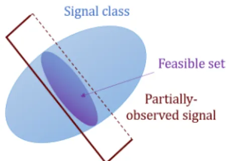
Figure 2.1: Feasible set of estimators.

geometric approach rather than a statistical one. We define the projection operator of a matrix Y onto an index set Ω by

[PΩ(Y)]ij =

(

Yij if Ωij = 1

0 if Ωij = 0

.

We use the subscripted vector (·)f o to denote fully observed data points

(columns), or data points with no missing values, and we use the subscripted vector (·)po to denote partially observed data points. We use a subscripted

matrix (·)f oor (·)poto denote the set of all fully observed or partially observed

data columns in the matrix.

We can impute a partially observed vector vpo by observing where its

ob-served samples intersect with the clusters C1, ..., Ck. Let the missing values

plane be the restriction set over _RF that satisfies the constraints on the observed values of vpo. We call this intersection thefeasible set W:

W ={ˆvpo∈Ck:PΩ(ˆvpo) = PΩ(vpo)} for some k ∈[K]. (2.4)

Fig. 2.1 illustrates the feasible set of a three-dimensional vector with two missing samples when the signal class (convex space containing samples from

kth cluster) covers an ellipsoid. If the signal had only one missing sample, the feasible set would be a line segment.

All k for which (2.4) is satisfied are possible clusters from which the true

v originated. Since W cannot be empty, there must be at least one Ck that

has non-empty intersection with the set of all points satisfying the PΩ(vpo)

(16)

over the feasible set of estimates: ˆ v_po∗ = arg min ˆ vpo∈Ck max v∈Ck kˆvpo−vk, (2.5)

where k · k denotes some norm or error function. If we use the ∞-norm, ˆv∗_po

is the Chebyshev center of the feasible set.

IfW contains estimators belonging to more than oneCk,W can be

parti-tioned into K disjoint sets,Wk,defined as

Wk={ˆvpo∈Ck :PΩ(ˆvpo) =PΩ(vpo)}, k∈[K]. (2.6)

Feasible clusters are those for which Wk is not empty, and we can find (2.5)

over the Ck for which the corresponding Wk covers the largest volume: k =

arg maxk|Wk|.

2.4.2

Application to non-negative matrix factorization

Let V ∈ _RF₊×N be a matrix of N sample points with F non-negative obser-vations. Suppose the columns in V are generated from K clusters. There exist W ∈ _RF×K

+ and H ∈ R

K×N

+ such that V = WH. This is the NMF of V [38]. We use the conical interpretation of NMF [35, 36], described as follows.

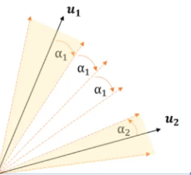
Suppose the N data points originate from K cones. We define a circular cone C(u, α) by a direction vector uand an angle α:

C(u, α) := x∈_RF_\{0}_: x·u kxk2 ≥cosα , (2.7) or equivalently, C(u, α) := x∈_RF_\{0}_{: (}_x_·_u₎2₋₍_x_·_x_{) cos}2₍_α₎_≥₀ _. _(2.8) We truncate the circular cones to be in the non-negative orthantP so that we haveC(u, α)∩P. We can considerukto be the dictionary entry corresponding

to Ck and all x’s belonging to Ck as noisy versions of uk. We call the angle

(17)

Figure 2.2: Geometric assumption for greedy clustering.

Figure 2.3: Decomposition of vectors in a circular cone. well-separated cones, that is,

min

i,j∈[K],i6=jβij >i,j∈max[K],i6=j{max{αi + 3αj,3αi+αj}}. (2.9)

This implies that the distance between any two points originating from the same cluster is less than the distance between any two points in different clusters, which is a common assumption used to guarantee clustering perfor-mance [36, 39, 40] (see Fig. 2.2). We can then partitionVintoksets, denoted

Vk :={vn ∈ Ck∩P}, and rewrite Vk as the sum of a rank-one matrix Ak

(parallel touk) and a perturbation matrixEk(orthogonal touk). For any

vec-tor z∈Vk,z=kzk2(cosβ)uk+y, where kyk2 =kzk2(sinβ)≤ kzk2(sinαk).

We use this rank-one approximation to find error bounds [36] (see Fig. 2.3). IfVcontains missing values, we can use the optimal recovery estimator to impute V. Assuming the columns in V come fromK circular cones defined as (2.7), there is a pair of factor matrices W∗ ∈ _RF×K₊ ,H∗ ∈ _RK×N₊ , such that

kV−W∗H∗kF

kVkF

≤max

k∈[K]{sinαk}. (2.10) Since the error is bounded by sinαk, we choose our optimal recovery

(18)

(2.8): ˆ v_po∗ = arg max ˆ vpo∈Ck {(ˆvpo·uk)2 −(ˆvpo·vˆpo) cos2(αk)}. (2.11)

We can solve (2.11) analytically using the Lagrangian with known values of vpo as equality constraints. We can also solve (2.11) numerically using

projected gradient descent.

Generally, uk is not known beforehand, but we can find uk given Wk.

Given an ellipse in_R3, we reconstruct its cone by drawing lines from its limit points to the origin. Then it is straightforward to find the center of the cone. Liu and Tan propose the following optimization problem (in the absence of missing values) over the optimal size angle and basis vector for each cluster [36]. We write the data points in each cluster as X:= [x1, . . . ,xM]∈RF+×M where M ∈_N+:

minimize(0,π/2) α

subject to xT_mu ≥cosα, m∈[M],

u≥0, kuk2 = 1, α≥0.

(2.12)

Of course, we also do not know Ck or Wk, so we use a clustering algorithm

to find the vectors belonging to each Ck (see Sec. 2.5).

2.5

Algorithm and error bound

Now we considering clustering and NMF with missing values. If the geometric assumption (2.9) holds, a greedy clustering algorithm [36, Alg. 1] returns the correct clustering of fully observed data. Here we show that a greedy algorithm also guarantees correct clustering of partially observed data under certain conditions.

Lemma 1 (Greedy clustering with missing values). Let Ωindicate the miss-ing values of vpo. Let αk be the defining angle of Ck and PΩ(αk) be the

defining angle of the cone resulting from projectingCk onto the missing value

plane from Ω. If, for exactly one k, arccos PΩ(vpo)·PΩ(uk) kPΩ(vpo)kkPΩ(uk)k ≤PΩ(αk) (2.13)

(19)

Algorithm 1: Greedy Clustering with Missing Values

Data: Data matrix V∈_RF×N

+ , K ∈N, Ω∈ {0,1}F×N

Result: Cone indicesJ ∈ {0,1, ..., K}N_;_α _∈₍₀_{, π/}₂₎K_; _u_∈

RF+×K

1 Partition columns inV into subsetsVf o and Vpo, where Vf o contains

data columns for which P

irij =F, and Vpo contains remaining

columns.;

2 NormalizeVf o so that all columns have unit `2-norm. Let V0f o be the

normalized matrix ;

3 Cluster items in V0_{f o} using greedy clustering [36, Alg. 1] to obtain

cluster indices J and run Alg. 3 on V0_{f o} to get u1, ..., uk fromW∗. ; 4 for v_po∈V_po do

5 Let Ωj correspond to observed entries of vpo. Find

k = arg maxj∈[K]cos−1

_P_Ω(_z

j)·PΩ(v)

kPΩ(zj)kkPΩ(v)k

. If this condition is maximized by more than one k, choose one at random. Add the index of vpo to Jk. ; 6 end 7 for k ∈[K] do 8 αk= maxvpocos −1 PΩ(vpo)·PΩ(uk) kPΩ(vpo)kkPΩ(uk)k ; 9 end

(20)

then vpo originated from the corresponding Ck. If αk are identical for all k,

Alg. 1 will cluster vpo correctly.

Proof. The result follows directly.

Now consider feasibility of imputing data points using the ˆα and ˆu from Alg. 2. Clearly, the missing values plane for each point intersects the original corresponding cone defined by the true u and α of the cone. We know the ˆu

fall somewhere within the original cones, but if the ˆα are too small, the new cones may not intersect with the missing values plane.

Lemma 2 (Feasibility of imputation algorithm). The estimator in (2.5) is able to find an imputation within the feasible set given α1, . . . , αK and

u1, . . . , uk returned by Alg. 1.

Proof. Let vector vpo be a partially observed version of vf o ∈ V. We define

the angle between vpo and cluster center uk in the F-dimensional space:

γk= arccos PΩ(vpo)·uk kPΩ(vpo)kkukk , (2.14)

and between vpo and the projected cluster center in the projected (F −f

)-dimensional space: ˆ γk = arccos PΩ(vpo)·PΩ(uk) kPΩ(vpo)kkPΩ(uk)k , (2.15)

where Ω is the observed values indicator corresponding to vpo. Thenγk≤γˆk

since PΩ(vpo)·uk =PΩ(vpo)·PΩ(uk) and kukk ≥ kPΩ(uk)k. Thus ˆγk is large

enough that an imputation on the missing values plane is feasible for each

vpo. Since αk= maxγk,all partially observed points labeled as belonging to

Ck can be imputed.

Algorithm 2: Rank-1 NMF with Missing Values

Data: Partially observed data V∈_RF×N

+ , Ω∈ {0,1}F×N, K ∈N

Result: Wˆ ∗ ∈_RF×K

+ and ˆH∗ ∈R

K×N

+

1 Cluster data using Alg. 1 ; 2 Impute data using (2.5) ;

(21)

We extend bound (2.10) on the relative NMF error to missing values (Alg. 3). Note that the original bound allows for overlapping cones and does not assume (2.9) holds. It only requires all points be within αk of uk,

which essentially allows the normalized perturbation matrix Ek to be

upper-bounded by sinαk. If the missing entries of eachvpoare imputed using Alg. 1,

then the perturbation from the original uk, which we denote ˆEk, will be at

most 2Ek. We can prove this using a worst-case scenario.

Theorem 1 (Rank-1 NMF with missing values). Suppose V is drawn from

K cones and missing values are introduced to get Vpo. If Alg. 2 correctly clusters data points and Alg. 1 is used to perform imputation, then

kV−W∗_poH∗_pokF

kVkF

≤max

k∈[K]{sin 2αk}, (2.16) where W∗_po and H∗_po are found by Alg. 3.

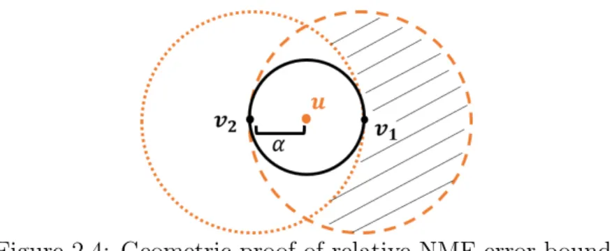
Proof. Suppose there are two points v1 andv2 in a cone, as indicated by the solid circle in Fig. 2.4. Thenuwill be at an angleαfrom bothv1andv2. Now suppose v2 contains missing values. Then the new v1 will be the only vector in the cone, ˆv2 is imputed using (2.11), where ˆu=v1,and ˆv2 is at an angular distance sin 2αfrom ˆu. (One can check that if there are more than two points in the cone, this distance cannot increase.) A worst-case imputation places ˆ

v2 at an angle 2α away from v1 (suppose the optimizer places ˆv2 at an angle greater than 2α fromv1, but this is a contradiction since then v2 would be a better estimate than the optimum). The dashed circle in Fig. 2.4 represents points at an angle 2α fromv1. Any ˆv2 outside the dotted circle is at an angle greater than 2α fromv2. So the shaded region indicates when the error may be greater than sin 2α. But the missing values of v2 allow for “movement” only along the axes. Since the intersection of a hyperplane with a cone is a finite-dimensional ellipsoid [41, 42], which is compact [43],v2 cannot “travel” via imputation to the shaded region without crossing a feasible region less than 2α from ˆu.Hence the theorem holds and is tight.

(22)

Figure 2.4: Geometric proof of relative NMF error bound.

2.6

Experimental results

To test our algorithm, we first generate conical data satisfying the geometric assumption, using N = 10000, F = 160, and K = 40. We choose squared length of each v as a Poisson random variable with parameter 1, and we choose the angles of v uniformly. We then let V be partially-observed with Bernoulli parameter ξ to obtain Vpo. That is,

Ω(i, j)i.i.d.∼ Bern(ξ). (2.17)

We run tests using ξ ∈ {0.4,0.55,0.7,0.8,0.9} and find imputation relative error for NMF: E[V,W∗_poH∗_po] = kV−W ∗ poH ∗ pokF kVkF . (2.18)

Fig. 2.5 shows relative error of our optimal recovery imputation with different values ofαwhen we enforce correct clustering. The error for allαvalues and missingness percentages lies within the bound given by (2.16). Note that because our data is drawn uniformly at random, the error does not approach the worst-case bound.

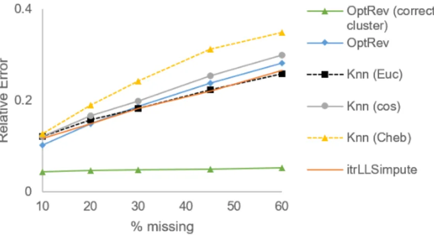
In the next experiment, we impute the conical data withα = 0.1 with other local imputation algorithms, including kNNimpute [44] with Euclidean, co-sine, and Chebyshev (L∞) distances and iterated local least squares (itrLLS)[45].

We perform two tests with optimal recovery: one with enforced correct clus-terings and one without prior knowledge of the correct clusclus-terings. We use

α = 0.1 and do not enforce correct clustering for Alg. 3 as before (see Fig. 2.6). We find k = 8 neighbors gives us the best results. Optimal recovery performs much better than other methods when clusters are known, and it performs similarly to other methods when they are not.

(23)

Figure 2.5: Relative NMF error of imputed conical data with correct clustering.

Figure 2.6: Relative NMF error for Conical data.

imaging data set from Pavia [46]. We crop the 103 images to have 2000 pixels per image, set K = 9,corresponding to the different imagery categories, and introduce missing values in the same proportions as before (see Fig. 2.7). We also run tests with mice protein data [47] (see Fig. 2.8). The original dataset contains 1077 measurements with 77 proteins. We remove the 9 proteins that had missing measurements, then introduce missing values. We find

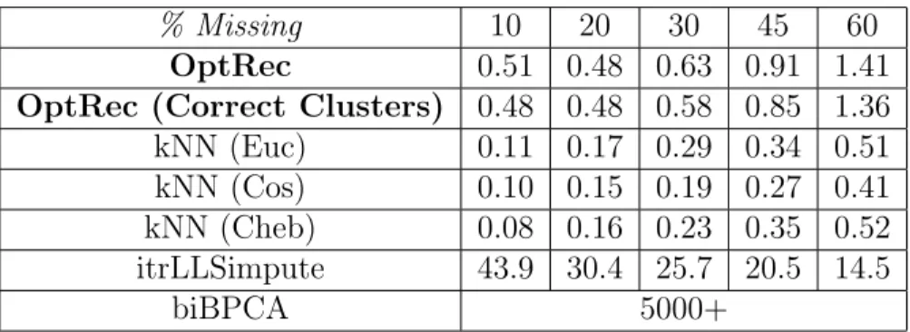
k = 5 neighbors gives us the best results for kNNimpute on these datasets. On the mouse data, we also test bicluster BPCA [30] in addition to the other methods. The conical and Pavia test data were not sufficiently well-conditioned to run bicluster BPCA. See Tab. 2.1 for a comparison of run times. Our results demonstrate that optimal recovery performs similarly to kNN methods when clusters are not known beforehand. When clusters are known, optimal recovery performs similarly to more advanced methods (itrLLSimpute and biBPCA) in a fraction of the time.

(24)

Figure 2.7: Relative NMF error for Pavia data.

Figure 2.8: Relative NMF error for Mouse data.

Table 2.1: Average imputation times for Mouse data in seconds.

% Missing 10 20 30 45 60

OptRec 0.51 0.48 0.63 0.91 1.41

OptRec (Correct Clusters) 0.48 0.48 0.58 0.85 1.36 kNN (Euc) 0.11 0.17 0.29 0.34 0.51 kNN (Cos) 0.10 0.15 0.19 0.27 0.41 kNN (Cheb) 0.08 0.16 0.23 0.35 0.52 itrLLSimpute 43.9 30.4 25.7 20.5 14.5

(25)

Algorithm 3: SVD with missing values

Data: Data matrix V(0) ∈RF+, K ∈N

Result: U∈_RF×K_,_Σ_∈

RK×K,X∈RK×N

1 InitializeU₍₀₎,Σ₍₀₎,X₍₀₎ ;

2 for t= 1,2, ... until convergence do 3 M(t) =U(t−1)Σ(t−1)X(t−1) ; 4 V₍_t₎ =P_Ω(V₍t−1)) +PΩC(M₍_t₎) ; 5 U₍_t₎,Σ₍_t₎,X₍_t₎=svd(V₍_t₎, K) ; 6 end 7 ReturnU(t),Σ(t),X(t) ; Algorithm 4: Rank-1 NMF

Data: Data matrix V∈_RF×N

+ , J ∈[K]N Result: U∈_RF×K_,_Σ_∈ RK×K,X∈RK×N 1 for k = 1 to K do 2 Vk:=V(:, Jk) ; 3 [U_k,Σ_k,X_k] := svd(Vk) ; 4 w∗_k :=|U_k(:,1)|,h_k:=Σ_k(1,1)|X_k(:,1)| ; 5 h∗_k:= zeros(1, N), h∗_k(Jk) :=hk ; 6 end 7 W∗ := [w∗₁, ...,w∗_K], H∗ := [(h∗₁)T, ...,(h∗_K)T] ; 8 ReturnW∗,H∗ ;

(26)

Figure 2.9: Minimum covering sphere in two dimensions.

2.7

Probabilistic error

We now make some probabilistic assumptions on our data and missingness patterns to calculate the expected maximum error of optimal recovery impu-tation. First, consider a coneC in anF-dimensional space defined byu and

α. Let us ignore the length of the vectors inC and preserve only the angles of the vectors from u. We can then represent vectors of an F-dimensional cone as points in an (F −1)-dimensional ball. For example, a 3-dimensional cone can be represented as points in a circle, as in Fig. 2.4.

Let there beN points{x1, ..., xN} ∈RF, drawn uniformly at random from

K F-dimensional balls, labeled B1, ..., BK. Let d(xi, xj) be the Euclidean

distance between xi and xj. We assume there is at least one data point in

each ball, and that the distance between any two points in a ball Bk is less

than the distance between any point in Bk and a point not in Bk:

For anyi, j ∈[N], i6=j, max i,j∈Bk d(xi, xj)< min i∈Bk,j /∈Bk d(xi, xj) for all k = 1, ..., K. (2.19)

This is equivalent to the geometric assumption in (2.9), and we can correctly cluster any points drawn from such balls using the greedy clustering algo-rithm already described. After obtaining the clusters, we can compute the minimum covering sphere (MCS) on the points in each cluster [48] (Fig. 2.9). This gives us K balls with Nk points in each ball.

Now suppose that we have partially observed entries in our data. Let the missingness of a point be a Bernoulli random variable with parameter

γ. That is, x is fully observed with probability γ and partially observed with probability 1−γ. There is now some uncertainly about the position

(27)

of partially observed data points, so we will find the MCS for only the fully observed points. This is analogous to step 3 in Algorithm 2. By calculating the expected change in the radius of the MCS, we can calculated the expected change in its corresponding cone.

If we assume the N points are drawn uniformly from the K balls, then

E[Nk] = N/k, and the expected number of fully observed and partially

ob-served points in each cluster is

E[|Xk,f o|] =γNk and E[|Xk,po|] = (1−γ)Nk. (2.20)

Clearly, the volume of the MCS can only decrease as|Xk,f o|decreases. Let

Rmax be the radius of MCS if there were no missing values, and let ˆR be the

radius of the MCS of only the fully observed points. Then ˆR < Rmax only

if any x ∈Xpo originally lay on the surface of MCSk,f o. Suppose the points

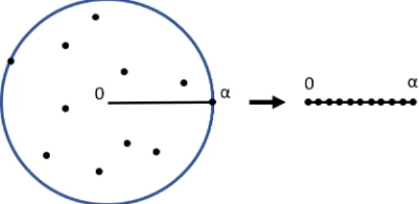
are randomly distributed along the radius of the F-ball and we pick points to be partially observed uniformly at random. Let

Npo=d(1−γ)Ne. (2.21)

Assume xi are i.i.d. and uniformly distributed (without loss of generality) on

[0,1]. This matches the assumption in the probabilistic analysis in [36] that the angles are drawn uniformly at random on [0, α] (see Fig. 2.10). Assuming a continuous distribution, almost surely no two points have exactly the same radius, and the probability of picking the ` outermost points is

P(`) = N−` Npo−` N Npo , where` = 0,1, ..., Npo . (2.22)

(28)

Figure 2.10: Assumption that points are uniformly random on the radius. This gives us E[`] = Npo X `=1 `·_P[`] (2.23) = Npo X `=1 `· N−` Npo−` N Npo (2.24) = _N1 Npo Npo X `=1 `· N −` Npo−` (2.25) = N−1 Npo−1 N(N + 1) N Npo (N −Npo+ 1)(N −Npo+ 2) , (2.26)

where Npo is dependent on γ, as defined in (2.21).

The radius of the resulting MCS is dependent on the distribution of points along the radius. We can determine ˆR using order statistics. If we assume uniform distribution between 0 and 1, and order the points x1, ..., xn so that

x1 is closest to the center of the sphere and xn is farthest, the radius of the

nth point, Rn, is given by the Beta distribution

Rn ∼B(n,1), (2.27)

and

E[Rn] =

n

n+ 1. (2.28)

Thus if ` of the outermost points are chosen to be missing,

E[ ˆR] =Rmax−(`/N)Rmax = N −` N Rmax . (2.29)

(29)

Figure 2.11: Example of _E[ ˆR] with N = 9 and`= 3.

since _E[`] is a function ofγ, we have derived the expected radius of the MCS as a function of missingness: E[ ˆR] = N −_E[`] N Rmax . (2.30)

Now we reverse the arrow in Fig. 2.10. Due to the random distribution of points in the sphere, removing the ` outermost points does not change the expected center u of the MCS. Transitioning from spheres back to cones, we get E[ ˆα] = N −_E[`] N α . (2.31) Thus α−_E[ ˆα] = E[`] N ·α, (2.32)

and the normalized Frobenius distance between W∗_{f o}H∗_{f o} and W∗H∗ for a single cone is:

kW_{f o}∗ H∗_{f o}−W∗H∗kF kW∗_H∗_k F ≤sin E[`] N ·α . (2.33)

If we assume vn ∈ V are MCAR, the statistical mean of Vf o is the same

as that of V. Since vn are uniformly distributed, the range of vn remains

centered on the mean, so the expected center of the MCS does not change. Thus the maximum difference between a pointv ∈Ck and its imputed point

ˆ

v is sinαk. Thus after imputing with Alg. 3, we can tighten the bound in

(2.16) to

kV−W_po∗ H∗_pokF

kVkF

≤ max

(30)

2.7.1

MCS with a different assumption

If instead we assume points are uniformly distributed in the volume of the ball, we find the change in radius as follows. First, calculate the volume of a

F-dimensional ball of radius R= 1:

VF(R) =

πF/2 Γ(F/2 + 1)R

F_. _(2.35)

Then we calculate radius ˆR of an F-dimensional ball as: ˆ RF( ˆV) = Γ(F/2 + 1)1/F √ π ˆ V1/F, (2.36) where volume ˆV = 1_N−` VF(1).

The probability that a pointx is in MCSpo is

P(x∈MCSpo) =

V( ˆR)

V(Rmax)

. (2.37)

Thus the expected radius given a missing parameter γ is given by

E[ ˆR] = ˆRF 1−_E[`] N VF(1) , (2.38) where _E[`] is a function of γ.

2.7.2

Minimum covering spherical cap for normalized data

If the data is normalized such that each vector has an L2 norm of 1, all the points will fall on the surface of a sphere. Let there beN points{x1, ..., xN} ∈

RF, drawn at random from K F-dimensional spherical caps of a radius R

F-ball, labeled C1, ..., CK. Let d(xi, xj) be some distance between xi and

xj. Assume there is at least one data point in each spherical cap, and that

Assumption 1 holds.

The area of an F-dimensional spherical cap is

A(R, h) = 1 2AFR F−1_I 2rh−h2/r2 F −1 2 , 1 2 , (2.39)

(31)

height of the cap, which can be calculated as a function of the angleαbetween the center and the edge of the cap, and Ix(a, b) is the regularized incomplete

beta function. Using the same style of analysis from the previous section, we can find the expected angle _E[αpo_{] given a parameter}_γ _{for partially observed}

points.

2.8

Conclusion

We have extended classical approximation-theoreticoptimal recovery for im-puting missing values, specifically for NMF. We showed that imputation using optimal recovery minimizes relative NMF error under certain geomet-ric assumptions. This required a novel reformulation of optimal recovery using the geometry of conic sections. Future work aims to extend optimal recovery to other settings of missing values in modern data science. On the experimental side, we plan to test our imputation algorithm on single-cell RNA sequencing data along with different clustering algorithms. We also aim to extend our algorithm to use local structure to take advantage of all observable data.

(32)

CHAPTER 3

MISSING VALUES AS NOISY CHANNELS

3.1

Introduction

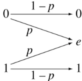
We can consider the missingness mechanisms described in Chapter 2 as dif-ferent types of channel noise. In the simplest case, MCAR mechanisms can be modeled as an erasure channel (Fig. 3.1). MAR and MNAR mechanisms can be modeled as signal-dependent noise channels. Ding and Simonoff de-scribe X missingness, or missingness that is dependent on observed variables (equivalent to MAR), M missingness, or missingness dependent on missing variables (equivalent to MNAR), and Y missingness, or missingness depen-dent on an output (such as signal class or some function of the signal obser-vations). Missingness can also be mixed (MX, MY, XY, XMY). Consider a case of MNAR missingness in gene testing where small gene counts are missed and recorded as zeros. This can be modeled as a channel that distorts or attenuates small signals with high probability and leaves large signals un-changed. One can define other similar signal-dependent or class-dependent erasure channels and derive channel capacities to obtain information the-oretic bounds. We use an erasure channel to model MCAR mechanisms, leaving the other mechanisms as an area for future work.

(33)

3.2

Missing values as a binary erasure channel: Fano’s

inequality and multiple hypothesis testing

Consider a set of n samples Y = (Y1, ..., Yn) drawn from joint

distribu-tion Pn

θ(y) parametrized by θ, where θ lies in some set Θ. If inputs X =

(X1, ..., Xn) are present, samples are drawn from joint distribution Pθ,Xn (y)

parametrized by (θ,X).An algorithm forms an estimate ˆθ ofθ, with the goal that some loss function `(θ,θˆ) is small.

We set up a multiple hypothesis test. Let V ∈ {1, ..., M} be an index corresponding to the parameters θV. Suppose V is drawn from a prior

dis-tribution PV, and a sequence of samples Y is drawn from PY|V. The goal

is to identify V with high probability given Y. If our estimation algorithm correctly outputs ˆθ ≈θV,then we should be able to recover the indexV from

ˆ

θ.This is the problem of multiple hypothesis testing, where the vth hypoth-esis is that the underlying parameter is θv. If the hypothesis test cannot be

successful, then the algorithm cannot perform well [49].

We use Fano’s inequality to lower bound the error probability. For exact recovery, we define error probability as

Pe =P[ ˆV 6=V]. (3.1)

Theorem 2 (Fano’s inequality). For discrete random variables V andVˆ on a common alphabet V,

H(V|Vˆ)≤H2(Pe) +Pelog(|V| −1), (3.2)

where H2(·) denotes the binary entropy. If V is uniform on {1, ..., M}, then

I(V; ˆV)≥(1−Pe) log|V| −log 2, (3.3)

or

Pe ≥1−

I(V; ˆV) + log 2

log|V| . (3.4)

Proof. The proof of (3.2) can be found in [50]. To get (3.3), we use|V| −1≤ |V| and H2(Pe) ≤ log 2, and we subtract H(V) = log|V| from both sides

[49].

(34)

inequality to bound I(V; ˆV) ≤ I(V;Y). If each of the n observations can take on b values, I(V;Y)≤H(Y)≤nlogb, so

Pe ≥1−

nlogb+ log 2

logM . (3.5)

Thus to achieve Pe≤δ, we need

n ≥ (1−δ) logM −log 2

logb (3.6)

samples. Suppose samples are missing completely at random with probability

ξ. The problem can be modeled as an erasure channel, and maxI(V; ˆV) is scaled by a factor of (1−ξ). Substituting (1−ξ)I(V; ˆV) forI(V; ˆV) in Fano’s inequality, we now need

n ≥ (1−δ) logM −log 2

(1−ξ) logb (3.7)

samples to achieve Pe≤δ.

For approximate recovery, the error probability is defined as

Pe(t) = P[d(V,Vˆ)> t], (3.8)

where d(v,vˆ) is some real-valued function and t ∈ _R. We define minimum and maximum neighborhood sizes

Nmax(t) = max

ˆ

v∈Vˆ

Nvˆ(t) and Nmin(t) = min

ˆ

v∈Vˆ

Nvˆ(t), (3.9) where Nvˆ(t) is the number ofv ∈ V for which d(v,vˆ)≤t.

Theorem 3 (Fano’s inequality with approximate recovery). For any random variables V and Vˆ on the finite alphabets V and Vˆ,

H(V|Vˆ)≤H2(Pe(t)) +Pe(t) log |V| −Nmin(t) Nmax(t) + logNmax(t). (3.10) If V is uniform on V, then I(V; ˆV)≥(1−Pe(t)) log |V| Nmax(t) −log 2, (3.11)

(35)

or equivalently, Pe(t)≥1− I(V; ˆV) + log 2 log _N|V| max(t) . (3.12)

Proof. The proof can be found in [51].

Again, we can use the data-processing inequality to bound I(V; ˆV) ≤

I(V;Y).If each of the n observations can take on b regions of values, where each region d(v,vˆ)≤t, thenI(V;Y)≤H(Y)≤nlogb, so

Pe ≥1− nlogb+ log 2 log _N|V| max(t) . (3.13) To achieve Pe(t)≤δ, we require n≥ 1 logb (1−δ) log |V| Nmax(t) −log 2 . (3.14)

To achieve Pe(t)≤δ with samples MCAR with probability ξ, we need

n≥ 1 (1−ξ) logb (1−δ) log |V| Nmax(t) −log 2 . (3.15)

3.3

Group testing with missing outcomes

We describe the group testing problem and directly apply (3.7) and (3.15) to existing bounds outlined in [49]. Suppose we have a set of p items. Of these items, k are defective. The set of defective items S ⊆ {1, ..., p} is uniform over the p_k possible subsets containing k items. For each test, a subset of the pitems are polled, and the test produces a binary outcome indicating if the polled subset contains at least one defective item. The goal is to identify

S with the fewest tests.

We denote the test matrix X ∈ {0,1}n×p _{where the} _X

i,j is 1 if item j is

included in test i. We let X be chosen in advance and randomly distributed (e.g., i.i.d. Bernoulli).

Scarlett and Cevher [49] consider passing the noiseless test outcome through a binary symmetric channel (BSC), which corresponds to incorrect test out-comes. In their model, the observed outcome is given by

(36)

Yi = _ j∈S Xij ! ⊕Zi, (3.16) where W

j∈SXij is the noiseless test outcome, ⊕ denotes modulo-2 addition,

and ∨is the “OR” operation. LetZi be i.i.d. Bernoulli() for some ∈[0,1₂)

and independent of X. Let the vector of test outcomes Y = {Y1, ..., Yn}.

Given X and Y, we estimate ˆS from ˆS. In the exact recovery setting, the probability of error is given by

Pe=P[ ˆS 6=S]. (3.17) Theorem 4 (Group testing under BSC with exact recovery). Under the noisy group testing setup described above, in order to achieve Pe ≤ δ, we

must have

n≥ klog

p k

log 2−H2()(1−δ−o(1)) (3.18) as p→ ∞, possibly with k → ∞ simultaneously.

Proof. We can directly formulate this problem as a multiple hypothesis test with V =S. Applying Fano’s inequality with conditioning on X, we obtain

I(S; ˆS|X)≥(1−δ) log p k −log 2. (3.19)

We upper boundI(S; ˆS|X)≤I(S;Y|X) using the data processing inequality, since S → Y → Sˆ when conditioned on X. Since the noise variables Zi

are independent, and Yi are conditionally independent of Xi and S given

W j∈SXij, we have I(S;Y|X)≤ n X i=1 I(_ j∈S Xij;Yi). (3.20)

Since Yi is generated from Wj∈SXij using a BSC, which has capacity log 2−

H2(), we have

I(S;Y|X)≤n(log 2−H2()). (3.21) Substituting the inequality p_k≥(p_k)k _{and (3.21) into (3.19) gives us Thm.}

(37)

Similarly, we can model the error using a BEC to obtain the following theorem. This would correspond to the case in which test outcomes are undetermined or missing with probability P.

Theorem 5 (Group testing under BEC with exact recovery). Under the group testing setup with missing test outcomes, in order to achieve Pe ≤ δ,

we must have n ≥ klog p k log 2−P (1−δ−o(1)) (3.22)

as p→ ∞, possibly with k → ∞ simultaneously.

Proof. The proof is similar to the proof of Thm. 4, except that the BEC has a capacity of log 2−P.

For the approximate recovery case, the decoder outputs a listL ⊆ {1, ..., p} of cardinality L≥k. We can then define

Pe(αk) =P[|S\ L|> αk]. (3.23)

In other works, if the number of missed defective items exceeds some fraction of the total number of defective items, then the decoder is wrong.

Theorem 6 (Group testing under BSC with approximate recovery). Under the noisy group testing setup with approximate recovery, with list size L≥k, in order to achieve Pe(αk)≤δ for some α∈(0,1), we need

n≥ (1−α)klog

p L

log 2−H2()

(1−δ−o(1)) (3.24)

as p→ ∞, k → ∞, and L→ ∞ simultaneously with L=o(p).

Proof. We apply Thm. 3. The number of L with cardinality L within a neighborhood αk of S is given by Nmax(αk) = bαkc X j=0 p−L j L k−j , (3.25)

which is the number of ways to place up toαkitems inL. Hence, conditioning on X and the data processing inequality as in Thm. 4, we get

I(S;Y|X)≥(1−δ) log

p k

(38)

Using some asymptotic simplifications (described in [49]), we combine (3.26) and (3.21) to obtain Thm. 7.

Again, this can be extended to a BEC corresponding to missing test out-comes.

Theorem 7 (Group testing under BEC with approximate recovery). Under the BEC group testing setup with approximate recovery, with list size L≥k, in order to achieve Pe(αk)≤δ for some α∈(0,1), we need

n≥ (1−α)klog

p L

log 2−P

(1−δ−o(1)) (3.27)

as p→ ∞, k → ∞, and L → ∞ simultaneously with L=o(p). Note that P

is the error rate of the BEC.

Proof. The proof is the same as that of Thm. 7 but with the BEC channel capacity.

In this example, we assumed i.i.d. Bernoulli missingness, corresponding to the MCAR case. To account for the MAR and MNAR cases, there has been some work on the capacity of signal-dependent noise channels [52], but this is an open area for future research.

(39)

CHAPTER 4

REGISTRATION FOR IMAGE-BASED

TRANSCRIPTOMICS: PARAMETRIC

SIGNAL FEATURES AND MULTIVARIATE

INFORMATION MEASURES

Image-based transcriptomics involves determining spatial patterns in gene expression across cells and tissues. Image registration is a necessary com-ponent of data analysis pipelines that characterize gene expression levels across different cells and intracellular structures. We consider images from multiplexed single molecule fluorescent in situ hybridization (smFISH) and multiplexed in situ sequencing (ISS) datasets from the Human Cell Atlas project and demonstrate a novel approach to groupwise image registration using a parametric representation of images based on finite rate of innova-tion sampling, together with practical optimizainnova-tion of empirical multivariate information measures.

4.1

Introduction

The transcriptome of a cell (or an organism) is the portion of DNA that is expressed as RNA in that cell (or organism). The subset of genes that are expressed in a cell varies depending on cell type and cell state, and recognizing patterns in the transcriptome is an important part of understanding cell function and pathology. The RNA molecules present in a cell can be tagged using fluorescent markers, which can be observedin situ, and spatial patterns of gene expression within cells and tissues can be studied [53]. Different combinations of colored fluorescent markers serve as tags for different RNA sequences, and images of different color spectra (multispectral images) must be aligned for analysis.

Researchers have developed methods and algorithms to extract transcript molecule feature sets, localization, and patterns, in tens of thousands of single cells across the human transcriptome [54, 55]. Starfish, a community of computational biologists and software engineers, has developed standardized

(40)

file formats for input data and analysis [56]. They are building a standard library that consolidates different methods from different steps of the analysis pipeline. The goal is to contribute to the Human Cell Atlas, a project to create comprehensive reference maps of all human cells to understand human health and to diagnose, monitor, and treat disease [57].

An important part of the image-based transcriptomics analysis pipeline is image registration. Image registration in the Starfish pipeline currently addresses pixel-level translational error using an FFT-based phase correla-tion approach [58]. Phase correlacorrela-tion has also been extended to rotacorrela-tional and scaling error [59] as well as to subpixel registration [60]. However, phase correlation does not account for non-linear intensity changes, which can arise when the images to be registered are taken under different conditions (e.g. multimodal, multispectral, different lighting, etc.). To address such intensity nonlinearities, mutual information has been proposed elsewhere as an image similarity measure [61, 62], and under the assumption that images are sta-tistically dependent, we have shown that maximizing mutual information is a theoretically optimal method for registering image pairs [63].

What about registering not just a pair of images but a larger set of images, as in transcriptomics? A natural extension to mutual information is multiin-formation, which can be used to jointly register multiple images and has been shown to be superior to sequential pairwise registrations and asymptotically optimal [63]. However, computing the multiinformation of several images is computationally expensive—O(Nn_{) for} _n _{images with} _N _{pixels. To address}

this computational issue we develop a novel parametric signal representation for image-based transcriptomics data using finite rate of innovation sampling [64]. We propose a feature- and information-based method which is O(nN) for n images. This algorithm registers images in a joint rather than pairwise manner and has the same output as multiinformation in certain settings when features are properly extracted; see Thm. 8 for a formal statement.

(41)

4.2

Registration using information

4.2.1

Mutual information

Maximizing empirical mutual information for image registration [61, 62] has been commonly used in fields such as medical imaging and remote sensing. Mutual information between random variables X and Y is defined as

I(X, Y) =H(X) +H(Y)−H(X, Y), (4.1) where H(X) and H(Y) are marginal entropies and H(X, Y) is the joint entropy of X and Y. Mutual information can also be formulated as the Kullback-Liebler divergence (relative entropy) between the joint distribution and the product of the marginal distributions:

I(X;Y) =X x,y pX,Y(x, y) log pX,Y(x, y) pX(x)pY(y) . (4.2)

Given two r-dimensional images X1 and X2 defined over a discrete spa-tial region Ω, we define an image transformation T : Ω → Ω. If X2 is a transformed version of X1,we can register X1 and X2 by finding

T∗ = arg max

T

I(X1(x, y);X2(T(x, y))). (4.3) There are several ways to estimate the joint and marginal distributions of images. Two popular ones are the joint histogram method [65] and the Parzen windowing method [66, 61]. After estimating the distributions, the maximization problem (4.3) can then solved using an appropriate optimiza-tion algorithm. If properly initialized, a local optimizaoptimiza-tion algorithm such as gradient descent can be used [65]. Global optimization algorithms such as genetic algorithms, simulated annealing, and particle swarm optimization have also been used to maximize mutual information [67, 68, 69, 70].

4.2.2

Multiinformation

Several groups have proposed using multiinformation to perform groupwise registration [71, 72, 73]. Guyader et al. show that groupwise

(42)

multiinforma-tion yields better registramultiinforma-tion performance than pairwise mutual informamultiinforma-tion for medical imaging settings. Multiinformation, like mutual information, is defined as the KL divergence between a joint distribution and a product of marginal distributions. Given n random variables X1, X2, ..., Xn,

multiinfor-mation is defined as I(X1;X2;. . .;Xn) = n X i=1 H(Xi)−H(X1, X2, . . . , Xn) =Xp(x1, x2, . . . , xn) log p(x1, x2, . . . , xn) p(x1)p(x2)· · ·p(xn) . (4.4)

To registernimagesX1, X2, . . . , Xn, we find the transformations that

max-imize multiinformation:

T₂∗, . . . , T_n∗ = arg max

T2,...,Tn

I(X1(x);X2(T2(x));. . .;Xn(Tn(x))), (4.5)

where x = (x, y) for a 2-D image. Thus a single optimization can be used to register any number of images. We call this the MM algorithm. We have recently shown that MM is exponentially consistent for image registration (probability of error goes to 0 exponentially fast as number of pixels goes to infinity) [63]. In fact, we showed that MM is asymptotically optimal in the sense of achieving the same error exponent as maximum likelihood registration. Thus T∗_{M M} =. T∗_{M L} = arg max T1,...,Tn n Y i=1 P(Xi(Ti(x, y))|Xi), (4.6)

where “=” indicates equivalent error exponents..

Guyader et al. assume images are jointly Gaussian, which greatly simplifies the empirical distribution estimation [71]. This is usually not a valid assump-tion for natural images or image-based transcriptomics (although they show that it works for the images they tested). Kern et al. [72] use the approxi-mation

I(X1;X2;. . .;Xn)≈

X

i,j∈{1,...,n};i6=j

I(Xi, Xj). (4.7)

This approximation can greatly overestimate multiinformation in cases where mutual information of image pairs is large.

(43)

Rather than approximating the multiinformation function, we initially im-plement the original objective in (4.5) using full image histograms. We per-form our optimization using particle swarm optimization [74]. The details of our implementation are covered in Sec. 4.4.

4.3

Feature-based registration

4.3.1

Background and related work

While MM performs groupwise registration optimally [63], it is computa-tionally expensive. Feature-based algorithms tend to be more efficient. Many registration methods first extract features and then match only the extracted features across images. Others have used corner detectors and edge detectors for registration [75, 76]. Phase correlation in the Fourier domain is applied to these features to retrieve translations and rotations. A particularly success-ful method is based on Lowe’s scale-invariant feature transform (SIFT) [77]. SIFT extracts local scale-invariant features, called keypoints, from images. Key points are image features that are visually interesting (e.g., corners and curved edges), and feature matching and clustering is performed to detect and register objects. Numerous variants of SIFT have been used in multi-modal image registration (we reference just a few) [78, 79, 80, 81].

Baboulaz and Dragotti formulate feature-based registration as a finite rate of innovation problem, with applications in super-resolution [82]. They use a Canny-like edge detector and use the intersections of those edges (corners) as features. They then match corners across images using correlation and RANSAC methods (also used in SIFT) and demonstrate that exact registra-tion is possible using only the detected corners.

We apply finite rate of innovation sampling to multispectral registration by representing smFISH images as sums of delta functions. We demonstrate that these features alone are enough to perform registration. We also use this sparse representation in conjunction with MM to perform groupwise registration.

(44)

4.3.2

Finite rate of innovation sampling

Certain signals that have afinite rate of innovation (FRI) [64] can be written in the form

s(t) =X

k

ckφ(t−tk), (4.8)

where φ(t) is a known kernel and the number of tk values per unit time (the

rate of innovation) is finite. Then the innovative part of the signal lies in

ck. Given ck and tk, we can reconstruct s(t). Various kinds of filters can

be used to identify the innovative part of the signal, and the signal can be perfectly reconstructed using just these samples [83, 84]. Examples of FRI signals include delta trains and piecewise polynomials.

For a 2-dimensional image, we can write (4.8) as

s(x, y) = X

x0_,y0_∈_Ω

cx0_,y0φ(x−x0, y −y0). (4.9)

Baboulaz and Dragotti register multiview images using FRI sampling. They model images as sums of polynomials, using a B-spline sampling kernel [82]. The images captured by digital imaging technologies result from the point spread function (PSF) of a lens, which can be used as the sampling kernel φ(x, y) in (4.9). An object in space o(x, y) is filtered through the lens as

s(x, y) =o(x, y)∗φ(−x/T,−y/T), (4.10) whereT is the sampling period. For registration, we must obtain the features ofo(x, y) froms(x, y).This can be done by deconvolvings(x, y) with the PSF of the imaging system to give ˆo(p, q). The image ˆo(x, y) is then processed to extract the features of interest, giving us a weighted sum of spikes:

d(x, y) = X

x0_,y0_∈_Ω

cx0_,y0δ(x−x0, y−y0). (4.11)

For every feature, there will be a corresponding spike in each misaligned image. To perform groupwise registration, we group these features across images and find the transformations so that spikes corresponding to a feature have the same location in each image.

(45)

Figure 4.1: Example smFISH images. Columns are different color channels. Rows are imaging rounds.

4.4

Methods and experiments

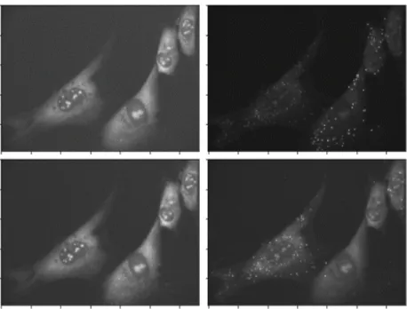
In this section, we demonstrate our algorithmic approach on manually shifted and rotated multispectral images, and then on a single smFISH image which we manually shift and rotate.1 _{Fig. 4.1 shows some example smFISH images.} Columns correspond to a color channel (there are three total), while rows corresponds to a round of imaging. Disturbances between imaging rounds may cause images to shift, and image registration is necessary. We perform a maximum intensity projection across channels to obtain one image per imaging round, and we perform registration with these images. In Sec. 4.4.3 we present our results on misaligned smFISH images, for which we do not have ground truth data.

4.4.1

Maximizing multiinformation

We implement MM using particle swarm optimization (PSO). To maximize (4.5), we must search over the spaceT2×T3×· · ·×Tn,where eachTi can have

multiple degrees of freedom. For example, if we restrict T to include only

1_{Code can be found at}

(46)

vertical and horizontal translations, each image has two degrees of freedom, giving us a 2n−1_{-dimensional search space. If we include rotations, it becomes} a 3n−1_{-dimensional search space. We can also include scaling, shearing, etc.} Clearly (4.5) is much more difficult to optimize than (4.3). We plot the multiinformation of 30 multispectral images from the CAVE database [85] with random horizontal and vertical shifts, estimating distributions using histograms (see Fig. 4.2). The maximum shift M is given on the x-axis, and images were shifted with a x-shift and a y-shift drawn uniformly on [0, M]. This matches the plots in [72] showing that mutual information of two images is maximized when they are properly aligned.

To test registration, we use five multispectral images, shown in Fig. 4.3. We randomly rotate them with angles between [−5,5] degrees. We find the em-pirical image intensity distributions for each image using image histograms, and compute the empirical joint distribution using a joint histogram. Using numerous histogram bins causes joint probabilities to become too small, so we use four bins. We calculate entropies and joint entropies using the empir-ical distributions, obtain multiinformation using (4.2), and maximize (4.3) using PSO. Because histograms are computationally expensive, we resized the images to decrease image sizes. We begin with exhaustive search of mul-tiinformation over all rotations and apply the transformation that maximizes multiinformation. (We restrict to rotations—only one degree of freedom per image—so we can test exhaustive search.) Comparing this to PSO yields the same results. Fig. 4.4 shows images transformed with shifts drawn uni-formly from [−10,10] pixels and rotations drawn uniformly from [−10,10] degrees. This example was initialized with 300 particles and converged after 211 iterations.

We also test a single maximum projection smFISH image; rather than re-sizing, we crop images and perform registration on areas with high densities of fluorescent markers. To increase the speed of PSO convergence, we use a dictionary to store the result of every computation so that the same calcula-tions need not be repeated, and we introduce a spread factor to the PSO to improve convergence speed [86].

(47)

Figure 4.2: Multiinformation of 30 multispectral images as a function of random shifts.

Figure 4.3: Top: Rotated test images. Bottom: Images registered using MM.

Figure 4.4: Top: Rotated and shifted test images. Bottom: Images registered using MM.

(48)

4.4.2

Finite rate of innovation sampling

If the weighted spikes corresponding to innovative features are correctly lo-cated across each image, the sampled spike images will be transformed ver-sions of the reference image, with transformations Tδ that are exactly the

original transformations T. If a spike δi has moved an L−2 distance less

than D from the reference spike δ1 for all images i = 2, . . . , n, and if any spike corresponding to a feature is significantly greater than distanceDfrom all other spikes in the image (that is, spikes are far apart and shifts and rota-tions were small), then we can use a nearest neighboring clustering algorithm to group spikes corresponding to the same feature across images.

We first demonstrate that we can register a collection of randomly shifted spikes. We randomly generate a 1000×1000 pixel image of 500 maximum intensity pixels (spikes) on a black background. We translate the image and use a nearest neighbor search to find where a spike has shifted. Both our algorithm and phase correlation register the images correctly with no error. We then add noise by randomly removing 50 spikes and randomly introducing 50 spikes. We then randomly shift individual spikes by 1 pixel to any of its eight adjacent locations. We find that both our algorithm and phase correlation produce an error of 1 pixel in any direction for about half of the images.

We test registration of multispectral images by randomly applying a ran-dom horizontal and vertical shift drawn from [−25,25], and we sample using Rosten and Drummond’s fast corner detection [87]. We represent corner lo-cations as spikes (see Fig. 4.5) and perform a nearest neighbor search using a search neighborhood of 30. FRI sampling followed by clustering again reg-isters the images correctly around 40% of the time, and is off by 1 pixel in any direction 60% of the time. On the other hand, cross-