Optimization of Reliability Allocation and Testing Schedule for Software Systems
Michael R. Lyu
Sampath Rangarajan
Aad P. A. van Moorsel
Bell Laboratories, Lucent Technologies
600 Mountain Avenue, Murray Hill, NJ 07974
f
lyu,sampath,aad
g@research.bell-labs.com
Abstract
To ensure an overall reliability of an integrated software system, software components of the system have to meet cer-tain reliability requirements, subject to some testing sched-ule and resource constraints. The system testing activity can be formulated as a combinatorial optimization prob-lem with known cost, reliability, effort, and other attributes of the system components. In this paper we consider the software component reliability allocation problem for a sys-tem with multiple applications. The failure rate of compo-nents used to build the applications are related to the testing cost through various types of reliability growth curves. We achieve closed-form solutions to problems where there is one single application in the system. Analytical solutions are not readily available when there are multiple applica-tions; however, numerical solutions can be obtained using a non-linear programming tool. To ease the specification of the optimization problem, we develope a GUI front-end to existing mathematical software. We present a systematic outline of the problem formulation and solution, and apply this to an example of a telecommunication software system.
1. Introduction
Modern complex software systems are often developed with components supplied by contractors or independent teams under different environments. For systems integrated with such modules or components, the system testing lem can be formulated as a combinatorial optimization prob-lem with known cost, reliability, effort, and other attributes of the system components. The best known system relia-bility problem of this type is the series-parallel redundancy allocation problem, where either system reliability is maxi-mized or total system testing cost/effort is minimaxi-mized. Both formulations generally involve system level constraints on
allowable cost, effort, and/or minimum system reliability levels. This series-parallel redundancy allocation problem has been widely studied for hardware-oriented systems with the approaches of dynamic programming [7, 16], integer programming [8, 3, 13], non-linear optimization [19], and heuristic techniques [17, 4]. In [5] the optimal apportion-ment of reliability and redundancy is considered for multiple objectives using fuzzy optimization techniques.
Some researchers also address the reliability allocation problem for software components. The software reliability allocation problem is addressed in [21] to determine how re-liable software modules and programs must be to maximize the user’s utility, subject to cost and technical constraints. Optimization models for software reliability allocation for multiple software programs are further proposed in [2] using redundancies. These papers, however, do not take testing time of software components and the growth of their relia-bility into consideration. Optimal allocation of component testing times in a software system based on a particular soft-ware reliability model is addressed in [12], but it assumes a single application in the system, and the reliability growth model is limited to the Hyper-Geometric Distribution (“S-shaped”) Model [20].
In this paper we discuss a generic software component reliability allocation problem based on several types of soft-ware reliability models in a multiple application environ-ment. This is the first effort to apply reliability growth models for guiding component testing based on multiple ap-plications. We will also give the solution procedure for the single application environment, for general continuous dis-tributions, thus generalizing [12]. We examine the situation where software components may interact with each other, a condition not considered by other studies. We also include scenarios for fault-tolerant attributes of a system where some component failures can be tolerated. The problem specifi-cation and solution seeking procedure, as well as a software tool for the automatic application of this procedure, are pre-sented in this paper as an innovative mechanism to handle
the difficult yet important reliability allocation problem. Several real projects motivate us for this investigation. These projects are described in the following case studies.
Distributed Software Systems. Distributed telecom-munication systems often serve multiple application types, which execute different software modules, and have dif-ferent reliability requirements. For instance, in telephone switches, 1-800 calls require processing different from stan-dard calls, and similar examples exists in call centers, PBXs or voice mail systems.
During the testing of such systems, reliability is a prime concern, and adequate test and resource allocation are there-fore very important. In the example we discuss in Section 6.2 it will become clear that trustworthy reliability growth curves can help considerably in efficient testing and debug-ging planning of such systems.
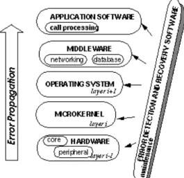
Fault-Tolerant Systems. Figure 1 shows a layered soft-ware architecture model that can be applied to many systems. Each layer can include several software components. Not all systems will necessarily include all the layers.
We conjecture that error propagation between layers only occurs in one direction, namely upwards. Thus, faults in the hardware that are not contained can propagate up to the oper-ating system or to the application software; however, faults not contained in the middle-ware layer will not propagate to the operating system but can propagate to the application software layer.
Error propagation occurs from layer
i
to layeri
+1 if layeri
has no fault tolerance mechanisms, i.e., the layer does not exhibit fail-silent behavior. From a modeling perspective, this layer would contribute higher failure rate to the overall system than a layer with error detection and recovery mech-anisms. Note that error detection and recovery software can reside in some or all of the layers.In Section 5.2 we will see how fault-tolerant mechanisms can be included in the reliability allocation problem formu-lation, provided that coverage factors are available.
Object-Oriented Software. Object-oriented software often allows for a clear delineation between different soft-ware components. If object-oriented softsoft-ware methods are being used, the relation between components and applica-tions can be assessed, and testing time can be assigned in the most efficient way.
Another optimization problem in object-oriented soft-ware testing arises when the best combination of objects must be selected to make an application as reliable as possi-ble. This optimization problem is an example of a ‘structure-oriented’ optimization problem, and can be solved by using methods presented in, e.g., [21, 2]. Our intent in this paper is
Figure 1. Layered software architecture
model.
to optimize with respect to software development and test-ing, not with respect to software structure. The combination of structure-oriented optimization methods in [21, 2] and the development-oriented methods in this paper can provide powerful tools in software system design.
The remaining sections of this paper are organized as follows: Section 2 specifies the optimal reliability alloca-tion as two related problems: a problem with fixed target failure rate, and a problem with fixed debugging time. The analytical solutions to these two problems are presented for the single application environment in Section 3: Section 3.1 for the exponential distribution, and Section 3.2 for gen-eral distributions. Section 4 discusses how the solutions for the problems in multiple application environment can be obtained. Our results are extended in Section 5.1 to con-sider software failure dependencies, and in Section 5.2 to incorporate fault-tolerant systems. Section 6 proposes the reliability allocation problem specification and solution pro-cedure into a step-by-step framework, and applies it to a case study. Section 7 describes the design and implementation of a software tool for systematic application of the reliability allocation framework. Conclusions are presented in Section 8.
2. Problem Specification
The above case studies can be described by a general problem of assigning failure-rate requirements (at the time of release) to software components that will be used to build various applications, given that the applications have pre-specified reliability requirements. Consider the situa-tion where a set of
N
software componentsC
1C
can be used in various combinations for different appli-cations. Let there be
M
such applicationsA
1A
M,
and let each application have a pre-specified reliability requirement
R
1(t
)R
M
(
t
). By investingdevelop-ment/testing/debugging time in components, component failure rates can be made such that all applications meet their reliability requirement.
Therefore, the goal in reliability allocation is to assign failure-rate requirements to the
N
components, such that all the pre-specified reliability requirements of theM
applica-tions are satisfied, at the minimal cost. In what follows, we will characterize the cost in terms of the component test-ing (includtest-ing debuggtest-ing) time. The optimization criterion thus is the minimization of this testing time. Furthermore, to relate the failure rate of components with the amount of testing time, we use reliability growth models.A variation to the above problem formulation arises if a fixed amount of testing time is available for each application. This requirement may occur because of the constraint on the cost incurred by the component developer and tester. In that case we take as objective function minimization of the failure rate of all the components.
In what follows we will continuously discuss these two variations of the optimization problem, and they will be referred to as the ‘fixed failure rate constraint’ problem and ‘fixed testing budget’ problem, respectively.
2.1. Fixed Failure Rate Constraint
In the fixed failure rate case, we assign testing time to components such that the applications meet their reliability requirements, and the testing time is minimized. Through-out this paper, we assume that the failure rates of components relate to the reliability of applications through the exponen-tial relation
R
i(
t
) =e
;it, where
i is the sum of failurerates of the components in application
A
ii
= 1
:::M
.Furthermore, we assume that the testing time
D
iinvested incomponent
i
decreases the failure rateiaccording to somereliability growth model. Note that we assume that once the software components are released, their failure rates stay constant. This is reasonable given that the application de-veloper does not debug or change the component that is used. In this context, we can formulate the allocation problem as follows.
The objective function is:
Minimize D
=D
1+D
2++D
Nsubject to the constraints:
111+122++1 NN 1(for applicationA
1), 211+222++2 NN 2(for applicationA
2), M11 + M22 ++ MNN M (for applicationA
M), where ij = 1 ifA
i uses component
C
j, and ij = 0 otherwise. Note1:::
N 0;D
1:::D
N 0; and 1:::
M0
:
For the sake of notational simplicity, weassume that the testing times
D
i are equally ’important’(costly) among the
N
components. If this is not the case one can apply weight!
ito each component testing timeD
iin the objective function.
Since a reliability growth curve can be very complex, the objective function is non-linear, and hence this is a gen-eral non-linear programming problem. In Section 3.1.1 we consider the closed-form solution for the problem with a single application, and in Section 4 we discuss the numeri-cal solution of the general case. Note also that we assume independence of components with respect to their failure behavior. This assumption may not be appropriate when software components may interact with each other, poten-tially causing additional failures.
2.2. Fixed Testing Budget
In the fixed testing budget case, we distribute per ap-plication a specified amount of testing time over its com-ponents, such that the application reliability is maximized. Consequently, the total failure rate of the components is the objective function to be minimized, leading to the following formulation as a mathematical programming problem. The objective function is:
Minimize
=1+2++ Nsubject to the constraints:
11D
1+12D
2++1 ND
Nd
1 (for applicationA
1), 21D
1+22D
2++2 ND
Nd
2 (for applicationA
2), M1D
1 + M2D
2 ++ MND
Nd
M(for applicationA
M), whered
1d
2d
M are the fixed amount of testing times
that are available for components used by applications
A
1A
2A
M, respectively. As in the previous problem,
all variables are positive. Weight functions for the failure rates
ican be introduced in the objective function to reflecttheir impact.
Of special interest is the single application case. This case corresponds to the optimization problem where all ap-plications together have a budget restriction on the testing time. The fixed testing budget problem is a variant of the fixed failure rate problem, and can be solved by similar means. In Section 3.1.2 and Section 4, we discuss the case of single and multiple applications, respectively.
3. Solutions for Single Application
Environ-ment
When there is only a single application in the system, an explicit solution of the reliability allocation problem can usually be found. In this section we give the general solution for a large class of reliability growth models (see Section 3.2). To explain the solution procedure, we first provide in Section 3.1 the solution assuming an exponential reliability growth model.
3.1. Exponential Reliability Growth Model
The exponential reliability growth model [9, 15] relates the failure rate
i(for componenti
) with the invested testingtime
D
ithrough: i = i0e
; i D i:
i0 is the initial failure rate at time 0, andi is the decayparameter. Over an infinite time interval i0
i
faults will be found. Note that
iis a function of time, although we do notexplicitly express it in the notation. This reliability growth model is in common use, and we will now determine the solution for the allocation problem in the single application environment.
3.1.1 Fixed Failure Rate Constraint
The fixed failure rate constraint problem can be formulated in the single application environment, assuming exponential reliability growth curves, as:
Minimize D
= N X i=1 1 iln
i0 i subject to: 1+2++ N:
To solve this, one can use the Lagrange method as follows [1]. The optimization problem is equivalent to finding the minimum of:
F
(1 N )=D
+((1++ N );)where
is a Lagrange multiplier. The necessary conditions [1] for the minimum to exist are:1. ∆(
F
(1 N))=0 where∆is the partial
deriva-tive operator, 2.
>
0,3.
1+2++ N=
.If we expand the equation from the first condition and take the partial derivatives w.r.t
1,2,,N, we can get
the following equations, respectively.
;1
11 +=0 ;1 22 +=0 ;1 NN +=0:
Given that the
and thevalues are all positive, it is clear that>
0, satisfying the second condition. From the above equations we also note that11 =22 ==N
N.Together with this observation and the third condition, we get the following solution for the obtained failure rates.
1= 1+ 1 2 ++ 1 N 2= 1 2 1 N = 1 N 1:
The testing times that should be allotted to the software components now follows from substituting the above values into the equations for
D
1,D
2,,D
N. For example,
D
1is equal toD
1= 1 1 ln 10 1+ 1 2 ++ 1 N:
Note that
D
1is positive if110:
To assure that noimpos-sible solutions arise, we present in Section 3.2 a procedure that checks for validity conditions and guarantees that the optimal solution follows a valid strategy.
Example 1: Consider an example where a system has three components
C
1,C
2, andC
3 and one applica-tionA
which uses all the components. All the three components have an initial failure rate of 5 failures/year (10 = 20 =30 = 5=yr
). Assume that the applicationrequirement states that the failure rate of the application (
) cannot be more than 6=yr
. Also assume that all the val-ues are the same and equals 1. In this case, we note that 1=2=3=2=yr
andD
1=D
2=D
3=ln(2:
5). Thatis, when the initial failure rates and the rate of reduction in failure rates with debugging is the same for all the compo-nents, then an average testing policy, where all the com-ponents’ failure rates are brought down to the same value, provides a solution that meets the application requirement with minimum testing time spent; the testing time spent on each component is the same.
Example 2: Now consider an example where the three components have initial failure rates which are different (say,
10=5=yr
,20=6=yr
,30=7=yr
). Assume that =6=yr
. Also assume that thevalues are all identicaland equal to 1. In this case, again we find that the required
values are the same and equal 2. Here again, an averagetesting policy provides a solution that meets the application
requirement with minimum testing time spent. But now, the testing time spent on each component is different because the initial failure rates are different. In this case,
D
1 =ln(5 2),
D
2 = ln( 6 2) andD
3 = ln( 72). The testing time spent on
each component is now proportional to the logarithm of the initial failure rate.
Example 3: Let us now assume that the three components have initial failure rates which are the same (
10 =20 = 30=5=yr
), and that thevalues are different (say,1=1, 2 = 2, 3 = 3). Again, assume that = 6. Now,computation tells us that to minimize the testing time, we require
1 = 6 1:834 = 3:
273, 2 = 3 1:834 = 1:
636 and 3 = 2 1:834=1
:
091. The optimal testing policy that leadsto the above failure rates will require a total testing time of ln( 51:834 6 )+ 1 2ln( 51:834 3 )+ 1 3ln( 51:834 2 )=1
:
49. Anaverage testing policy which assigns
1 = 2 = 3 = 2leads to a total testing time of ln(
5
2)1
:
834=1:
68 whichis more than that of the optimal testing policy.
3.1.2 Fixed Testing Budget
The fixed testing budget problem can be formulated in the single application environment, assuming exponential reli-ability growth curves, as:
Minimize
=1+2++ Nsubject to the constraint
D
1+D
2++D
ND:
Again, this can be solved using the Lagrange method, which uses that the optimization problem is equivalent to finding the minimum of
F
(D
1D
N )=+((D
1+D
2++D
N );D
)where
is the Lagrange multiplier. Again, the necessary conditions for a minimum to exist are:1. ∆(
F
(D
1D
2D
N)) = 0 where∆ is the partial
derivative operator, 2.
>
0,3.
D
1+D
2++D
N=
D
.If we expand the equation from the first condition and take partial derivatives with respect to
D
i, we get: i0 (;i
e
;iDi)+
=0:
Given that
i is positive, we note thatis positive andhence the second condition is satisfied. Thus, from the above equation, we get
10(;1e
;1D1 )=20(;2e
;2D2 ) == N0 (; Ne
;NDN ):
Using the above equation together with the constraint that
D
1+D
2++D
N =D
, we getD
1=D
; 1 2 ln( 202 101 )+ 1 3 ln( 303 101 )++ 1 N ln( N0 N 101 )] 1+ 1 2 ++ 1 ND
2 = 1 2 ln 202 101 + 1 2D
1D
N = 1 N ln N0N 101 + 1 ND
1:
The above equations determine how the testing times should be allocated to the different components. The min-imum
value that is obtained follows directly from the values for the testing times.It is interesting to note that only if the initial failure rates
i0’s and the i values are the same, an average testingpolicy where the available testing time is equally divided
among the components will provide an optimal solution. If either the
i0’s or the i values are different, then weneed to compute the above expressions to obtain an optimal allocation of the testing time.
Example 4: Consider the parameters from Example 3 where the initial failure rates are the same (
10 = 20 = 30 =5=yr
), and thevalues are different (say,1 =1, 2 = 2,3 =3). Assume that the available testing timeis 1yr. Then,
D
1 computes to 0:
1567,D
2 computes to 0:
4249 andD
3computes to 0:
4184. The optimized failure rate evaluates to1 = 4:
27=yr
,2 = 2:
14=yr
and3 =1
:
43=yr
for a total failure rate of 7:
84=yr
. If an average allocation policy is used, thenD
1=D
2 =D
3=0:
333 andthe failure rates evaluate to
1 = 3:
58=yr
,2 = 2:
57=yr
and
3 =1:
84=yr
for a total failure rate of 7:
99=yr
whichis worse than the optimal allocation. Let us try another allocation. Assume an allocation where
D
1 = 0:
4,D
2 =0
:
4 andD
3=0:
2. In this case, we note that1=3:
35=yr
, 2 =2:
25=yr
and3 =2:
74=yr
for a total failure rate of3.2. General Reliability Growth Models
In this section we provide the procedure to obtain the closed-form solution for generic reliability growth model. The only restriction to the growth models is with respect to the first and second derivatives. The solution procedure follows directly from the solution of the Lagrange method, except that impossible solutions must be prevented. It gen-eralizes the procedure for the hyper-geometric model given in [12] to general continuous distributions.
We consider the fixed failure rate constraint case. Let the relation between the failure rate and the testing time be given by some function
f
, that is:D
i =f
i ( i ):
Now, without loss of generality, the
N
components can be reordered according to the absolute values of the derivatives at the beginning of the debugging interval, at whichi=
i0:
That is:abs
(d
d
if
i ( i )j i=i0 )> abs
(d
d
i+1f
i+1 ( i+1 )j i+1= (i+1)0 )for
i
=12:::N
;1:
Using this ordering, the procedureto obtain the closed-form solution is as follows:
1.
K
=N
; 2. Fori
=1 toK
express i as a functiong
i ( K ) of K by equating d dif
i ( i )= d dKf
K ( K ); 3. Solve K from P K i=1g
i ( K )=; 4. If K>
K0 thenK
=K
;1 and goto step 2;else For
i
=1 toK
Compute i fromg
i ( K ) and the solution of K in step 3;The important feature in the algorithm is the ability to determine which component should be assigned zero testing time if an impossible solution is obtained (an impossible solution arises if
i>
i0for some component). If the firstderivatives d di
f
i (
i
)are less than zero for all
i
, and thesecond derivatives d d 2 i
f
i ( i)are greater than zero for all
i
, then it can be shown that the component ranked lowest according to the derivatives at time zero can be discarded. This happens in step 4 of the algorithm. In other words, the sufficient conditions on the derivatives say that the failure rate decreases over time, and that the rate of decrease gets smaller if time increases. Note that if the derivatives of the growth curve are less regular, specific conditions must be established to determine which components should not be assigned testing time.The above procedure can be similarly formulated for the fixed testing budget problem. We will not do so here.
Pareto Growth Model As an illustration, let us consider the Pareto distribution and consider the fixed failure rate constraint problem. The failure rate is given by
i(
t
) = i0 ( i1 +t
) ; i2, where
i0,i1andi2are constants. Hence,we have for the testing time:
D
i = i0 i i2 ; i1:
The Pareto class of failure-rate distributions is useful be-cause it is a generalization of the exponential, Weibull and gamma classes [11, 14].
One can show that the first derivative is less than zero, and the second derivative is greater than zero, provided
i0,i1and
i2are all positive. Hence, taking the partial derivativeof
D
iw.r.t. i, we get in step 2 of the algorithm (K
=N
inthe first iteration):
;
1 i2 i0 i2 ;( 1 i2 +1) i =; 1 K2 K0 K2 ;( 1 K2 +1) K:
In step 3, we have to equate the total failure rate to
:
In this case, we have to do that numerically, since a closed-form expression using the Pareto distribution is too intricate. As soon as we obtain a possible solution forK, we computethe individual failure rate using the relationship
i = i2 K2 1 K2 K0 1 i2 i0 ;( 1 K2 +1) K ! ;( 1 1 i2 +1 ):
Example 5: Assume the following parameters with Pareto distribution.
10 = 5, 11 = 1, 12 = 3, 20 = 2, 21 = 1, 22 = 6, 30 = 4, 31 = 1, 32 = 5. Theoptimal policy requires the following failure-rate values:
1=3:
395,2=1:
556,3=2:
047. The total testing timeis 0
:
3236.4. Solutions for Multiple Application
Environ-ment
When there are multiple applications in the system, the reliability allocation problem becomes too intricate to solve explicitly. However, in this case its solution can be obtained using non-linear programming software such as AMPL [6]. Let us here show how this procedure works for an example of a 3-component, 3-application system, by specifying and solving it using the RAT tool presented in Section 7.
Example 6: There are three components
C
1,C
2andC
3 which can be used to build three applicationsA
1,A
2andA
3.A
1is built usingC
1andC
2,A
2is built usingC
2andC
3andA
3 is built usingC
1,C
2, andC
3. Thus, there are multipleapplications, each with a failure-rate constraint. The fixed failure rate constraint problem can thus be formulated as:
Minimize D
=D
1+D
2++D
Nunder the constraints:
1+21(for applicationA
1), 2+32(for applicationA
2), 1+2+33(for applicationA
3).The fixed testing budget problem can be formulated as:
Minimize
=1+2++N
under the constraints:
D
1+D
2d
1D
2+D
3d
2D
1+D
2+D
3d
3:
Assume the parameters from Example 3 where the initial failure rates for the three components are the same (
10= 20 = 30 = 5=yr
), and the values are different (say, 1 = 1, 2 = 2, 3 = 3). Assume that the failure-raterequirements for the three applications are
1 =6,2 =5, 3=7. Modeling this as a non-linear optimization problemwith multiple constraints in AMPL and using the MINOS solver, we get the following result:
1=3:
818,2=1:
909and
3 = 1:
273. The total testing time for thisfailure-rate allocation evaluates to 1
:
207 yrs; (the individual testing times can be computed using the failure-rate allocation for each component). It is interesting to note that the failure-rate constraint forA
3 is strictly satisfied; forA
1 with the failure-rate requirement of 6=yr
, it is not strictly satisfied (1+2 = 5:
73), similarly forA
2 whose requirement is5
=yr
(2+3 =3:
18). Now consider an average testingpolicy where the constraint for the application
A
3is strictly satisfied without violating the other constraints. That is, 1 =2:
333,2 =2:
333 and3=2:
333. The total testingtime based on this average testing policy evaluates to 1
:
39 yrs, much larger than that obtained with the optimal testing policy.5. Software Failure Dependencies and
Fault-Tolerant Systems
The basic reliability allocation problem formulation can be extended in various ways. Here we discuss two exten-sions, software failure dependencies in Section 5.1 and fault tolerance aspects in Section 5.2.
5.1. Software Failure Dependencies
In the above discussions we assume software compo-nents fail independently. In reality, this may not be the
case. For example, the feature interaction problem[10] describes many incidents where independently developed software components interact with each other unexpectedly, thus causing unanticipated failures. We incorporate this ex-tra failure incidence by introducing pair-wise failure rates. Specifically,
ijrepresents the failure rate due to theinter-action of components
C
iandC
j, wherei
j
.The constraints of the original problem are then modified as:
111 + 122 + + 1 NN + P f8(ij)j1i=11 j =1g ij 1(for application A
1) 211 + 222 + + 2 NN + P f8(ij)j2 i =12 j =1g ij 2(for application A
2) M11 + M22 + + MNN + P f8(ij)j Mi =1 Mj =1g ij M (for application A
M ):
Subject to the above constraint we need to minimize
D
=D
1+D
2++D
N
:
The fixed testing-time problem can be obtained by adding the pair-wise failure rates in the objective function.
5.2. Fault-Tolerant Systems
In the situation where the system possesses fault tolerant attributes, we can introduce coverage factors [18] into the original problem. Coverage is defined as the conditional probability that when a fault is activated, it will be de-tected and recovered without causing system failure. With
c
idenoting the coverage measure for the componentC
iwecan reformulate the fixed failure rate constraint case, using
i =1;c
i, as:Minimize D
=D
1+D
2++D
N subject to: 1111+1222++1 NNN 1(for applica-tionA
1), 2111+2222++2 NNN 2 (for appli-cationA
2), M111 + M222 ++ MNNN M (for applicationA
M).6. Reliability Allocation Solution Framework
We have discussed the reliability allocation problem in terms of two constraints: fixed failure rates or fixed testing budgets. We also discussed the problem to account for
component interactions. The fault tolerant attributes in the system to tolerate component failures are also incorporated. In this section we describe a framework for specifying and solving a general reliability allocation problem, and describe how this procedure is applied to a specific application.
6.1. The Problem Specification and Solution Proce-dure
The following procedure specifies the reliability alloca-tion problem, and obtains solualloca-tions either analytically or using numerical methods.
1. Determine if it is a fixed failure rate constraint prob-lem or a fixed testing budget probprob-lem.
2. Determine if there is single application or multiple applications in the system.
3. Set the constraints on the failure rates or testing bud-gets.
4. Obtain parameters of the reliability growth curves of the components.
5. Determine if the components interact with each other. If so, obtain pair-wise failure rates.
6. Determine if there are fault tolerance features in the system. If so, obtain coverage measures for each component.
7. Format the problem as a non-linear programming problem with appropriate parameters.
8. If the solution is analytically available, obtain it. Oth-erwise, use the reliability allocation tool (see Sec-tion 7), based on the mathematical programming tool AMPL and solver MINOS, to obtain the results. In the following sub-section we examine a case study where a required reliability allocation problem is specified. We illustrate how the above procedure is applied to the project to obtain numerical solutions for various scenarios.
6.2. A Hypothetical Example
Let us consider a distributed software architecture that is used for switching telephone calls. Different call types will exercise different software modules, and we break up the system in components such that reliability growth models are available for all components. Of course, prerequisite to our analysis is the availability of reliable growth models, but the example will clearly show that it is beneficial to make decisions based on such models.
Table 1 shows the data input in this example. Neither the example nor the data corresponds to existing systems or numbers. We consider 4 types of calls (two types of standard calls, and two type of 1-800 calls), and 5 com-ponents (basic processing, scheduling, call processing, and two signal processing modules). The terms ‘in’ and ‘not in’ in Table 1 denote which components the applications use. For instance, the standard calls of type 1 use all software modules except the call processing module. The reliability growth curves for the components are exponential, and have parameters
and, as specified in the table.With the results obtained for this example, we want to show two things: the necessity to use mathematical optimization techniques to establish an optimal allocation scheme, and the importance of selecting and parameterizing adequate reliability growth models.
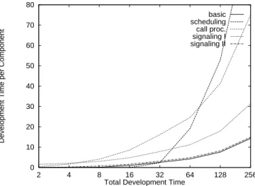
0 10 20 30 40 50 60 70 80 2 4 8 16 32 64 128 256
Development Time per Component
Total Development Time
basic scheduling call proc. signaling I signaling II
Figure 2. Total available testing time versus the optimal allocation for the components.
Figure 2 shows the total amount of testing time avail-able, versus the time allocated to the individual components. Following the framework in Section 6.1 we solved it as a fixed testing budget problem with multiple applications. We assumed, however, that the testing time is shared by all ap-plications, that is, we consider the special case mentioned in Section 2.2 where the constraints map to a single con-straint. Furthermore, applications are weighted based on their relative frequency of occurrence given in Table 1 (the RAT tool described in Section 7 automatically converts this to weights on the component failure rates in the objective function.) Using weights we thus include parts of the op-erational profile (see, e.g., Chapter 5 in [11]) in the model (see Table 1 for the relative frequencies of the different call applications). We obtained solutions for the testing time ranging from 2 to 256, and assumed no failure dependency or explicit fault-tolerant mechanisms. We input the problem
Component
i0 i standard I standard II 1-800 I 1-800 IIbasic 10 1.0 in in in in
scheduling 20 1.0 in in in in
call proc. 200 0.2 not in in in in
signal I 200 0.5 in in in not in
signal II 20 1.0 in in not in in
frequency 0.5 0.3 0.1 0.1
Table 1. System components with corresponding parameters growth curve, and applications that use the component.
in the RAT tool, and solved it using AMPL and MINOS. Figure 2 shows very clearly the dependence of the optimal schedule on the total testing time. For instance, while the scheduling component should not be assigned debugging time if a small budget is available, it takes the largest chunk if the testing budget is large.
The irregular assignment of testing time to individ-ual components in Figure 2 cannot be obtained easily by means other than mathematical modeling. With back-of-the-envelop calculations, one cannot expect to get such pre-cise results, and one would be bound to make inefficient decisions. 0.01 0.1 1 10 100 1000 10000 0.001 0.01 0.1 1 10 100
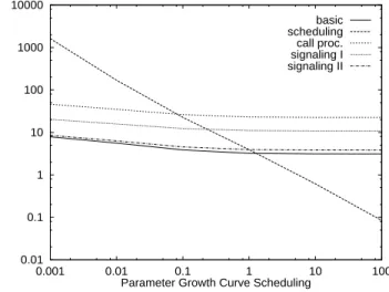
Development time per Component
Parameter Growth Curve Scheduling basic scheduling call proc. signaling I signaling II
Figure 3. Parameter
in growth curve ofscheduling software, versus the optimal al-location for all components.
Figure 3 shows the parameter
of the reliability growth curve corresponding to the scheduling software, versus the allocation of testing time to the components. In this case, we took the allowed failure rates per application to be 4, and solved the fixed failure rate constraint problem.Clearly, the parameter value greatly influences the
opti-mal solution. If the decay parameter of the reliability growth model of the scheduling component is small, it takes enor-mous investments in debugging time to reach the desired failure rates. If the decay parameter is relatively large, it takes minor effort for the scheduling component to obey to the failure rate restrictions.
The correlation between the optimal testing time and the parameters of the reliability growth curve shows the im-portance of data collection to establish trustworthy growth models. Without such models, decisions about reliability allocation are bound to be sub-optimal.
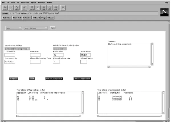
7. RAT: The Reliability Allocation Tool
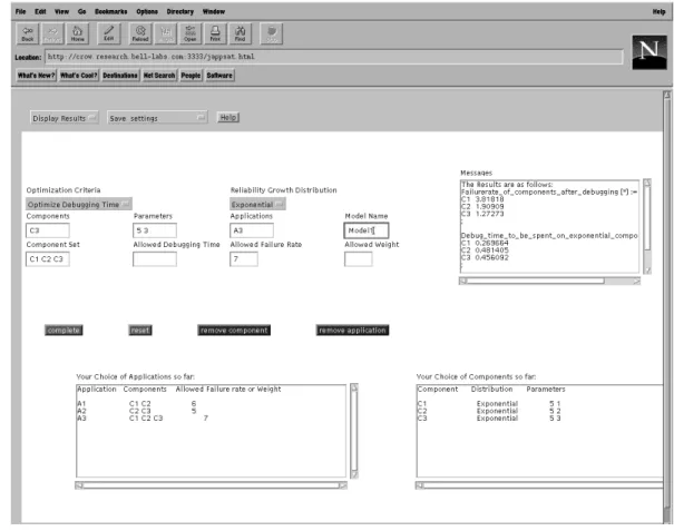
We have designed and built a reliability allocation tool (RAT) with a GUI based on a Java Applet. The tool allows multiple applications to be specified and allows optimiza-tions to be performed both under the fixed failure rate and fixed testing budget constraints. The user inputs the model using the GUI and the input is converted into AMPL files and is solved using the MINOS solver, called by AMPL. Figure 4 shows the GUI. The tool chooses the optimization criteria, where optimizing failure rate implies that the con-straint is fixed testing budget and optimizing testing time implies that the constraint is fixed failure rate. Components can be specified in the field named “Components” and appli-cations can be specified in the field named “Appliappli-cations.” The reliability growth distribution can be chosen for each components independently; parameters for these distribu-tions can be specified in the box named “Parameters.” At present exponential and Pareto distributions are allowed, but we plan to extend the options to specifying other distribu-tions. In case of a fixed-failure rate constraint, the allowed failure rate for the applications can be specified in the field named “Allowed Failure Rate”; similarly, if testing time is fixed, then this can be specified in the field named “Allowed Debugging Time.” Information about the components that have been specified and the applications that have been input are shown in two separate areas.
Figure 4. The reliability allocation tool.
As an example of the use of this tool, we consider the fixed-failure rate problem with multiple applications that we considered in Example 6. Figure 4 shows the interface after the components have been chosen and the configurations of the applications have been specified. In Example 6, there were three components
C
1,C
2andC
3each of which fol-lows an exponential reliability growth model with = 5and
values of 1, 2 and 3 respectively. This is shown in the area titled “Your Choice of Components so far.” Three applications are configured where applicationA
1uses com-ponentsC
1,C
2, applicationA
2usesC
2,C
3 and applicationA
3usesC
1,C
2andC
3. The applications have a failure-rate requirement of 6, 5 and 7 respectively. This is shown in the area titled “Your Choice of Applications so far.” This model when solved produces the result as shown in the "Message" area in Figure 5. As presented in Example 6, the results show that the failure rates ofC
1,C
2andC
3should be brought down to 3:
818, 1:
909 and 1:
273 respectively. This will minimize the total testing time used, while at the same time satisfying the failure rate requirements of all the appli-cations. The “Message” area also shows the testing times that need to be spent on each of the components to bring the failure rates of the components down to the above values. It is seen that the total testing time for the three components is as computed in Example 6.8. Conclusions
We consider the software component reliability alloca-tion problem for a system with single or multiple applica-tions, each with a pre-specified reliability requirement. The system testing activity is formulated as a combinatorial op-timization problem for overall system failure rate or testing time and cost. The relation between failure rates of compo-nents and cost to decrease this rate is modeled by various types of reliability growth curves.
We achieve closed-form solutions to problems with only one single application in the system, and we describe how to solve the multiple application problem using non-linear programming techniques. We also examine the interactions between the components in the system, and include inter-component failure dependencies into our modeling formula. In addition to regular systems, we extend the technique to address fault-tolerant systems. We further develop a proce-dure for a systematic approach to the reliability allocation problem, and describe its application in a case study. Finally, we present the design and implementation of a reliability al-location tool for an easy specification of the problem and an automatic application of the technique.
The presented methodology gives the basic solution ap-proach to the optimization of testing schedules, subject to
liability constraints. This adds interesting new optimization opportunities in the software testing phase to the existing optimization literature that is concerned with structural op-timization of the software architecture. Merging these two approaches will further improve the planning opportunities in software design and testing.
9. Acknowledgement
We wish to thank Chandra M. Kintala of Lucent Bell Labs. for many of his valuable suggestions and comments for this work.
References
[1] M. Avriel, ”Nonlinear Programming,” in
Mathemat-ical Programming for Operations Researchers and Computer Scientist, A. G. Holzman (Ed.), Chapter 11,
Marcel Dekker Inc., New York, 1981.
[2] O. Berman and N. Ashrafi,“Optimization Models for Reliability of Modular Software Systems,” IEEE
Transactions on Software Reliability, vol. 19, no. 11,
November 1993, pp. 1119–1123.
[3] R.L. Bulfin and C.Y. Liu, “Optimal Allocation of Re-dundant components for Large Systems,” IEEE
Trans-actions on Reliability, vol. R-34, 1985, pp. 241–247.
[4] D.W. Coit and A.E. Smith, “Reliability Optimiza-tion of Series-Parallel Systems Using A Genetic Al-gorithm,” IEEE Transactions on Reliability, vol. 45, 1996.
[5] A.K. Dhingra, “Optimal Apportionment of Reliability and Redundancy in Series Systems Under Multiple Objectives,” IEEE Transactions on Reliability, vol. 41, no. 4, December 1992, pp.576–582.
[6] R. Fourer et. al., “AMPL: A Modeling Language For Mathematical Programming,” The Scientific Press, 1993.
[7] D.E. Fyffe, W.W. Hines, and N.K. Lee, “System Re-liability Allocation and a Computational Algorithm,”
IEEE Transactions on Reliability, vol. R-17, 1968, pp.
64–69.
[8] P.M. Ghare and R.E. Taylor, “Optimal Redundancy for Reliability in Series System,” Operational Research, vol. 17, 1969, pp. 838–847.
[9] A.L. Goel and K. Okumoto, “Time-Dependent Error Detection Rate Model for Software and other Perfor-mance Measures,” IEEE Transactions on Reliability, vol. R-28, no. 3, August 1979, pp.206–211.
[10] N. Griffeth and Y.-J. Lin (ed.), IEEE
Communica-tions Magazine, Special Issue on Feature InteracCommunica-tions
in Telecommunications Systems, August 1993. [11] M. Lyu (ed.), “Handbook of Software Reliability
En-gineering,” McGraw-Hill and IEEE Computer Society Press, 1996.
[12] R.-H. Hou, S.-Y. Kuo, and Y.-P. Chang, “Efficient Al-location of Testing Resources for Software Module Testing Based on the Hyper-Geometric Distribution Software Reliability Growth Model,” Proceedings of
the 7th International Symposium on Software Relia-bility Engineering, October/November 1996, pp. 289–
298.
[13] K.B. Misra and U. Sharma, “An Efficient Algorithm to Solve Integer Programming Problems Arising in Sys-tem Reliability Design,” IEEE Transactions on
Relia-bility, vol. R-40, 1991, pp. 81–91.
[14] J. Musa, A. Iannino, and K. Okumoto, “Software Reliability: Measurement, Prediction, Application,” McGraw-Hill, 1987.
[15] J. Musa, “Validity of Execution-Time Theory of Soft-ware Reliability,” IEEE Transactions on Reliability, vol. R-28, no. 3, August 1979, pp. 181–191.
[16] Y. Nakagawa and S. Miyazaki, “Surrogate Constraints Algorithm for Reliability Optimization Problems with Two Constraints,” IEEE Transactions on Reliability, R-30, 1981, pp. 175–181.
[17] L. Painton and J. Campbell, “Genetic Algorithms in Optimization of System Reliability,” IEEE
Transac-tions on Reliability, vol. 44, 1995, pp. 172–178.
[18] D.P. Siewiorek and R.S. Swarz, Reliable Computer
Systems: Design and Evaluation, Digital Press, 2nd
edition, 1992.
[19] F.A. Tillman, C.L. Hwang, and W. Kuo, “Determining Component Reliability and Redundancy for Optimum System Reliability,” IEEE Transactions on Reliability, vol. R-26, 1977, pp. 162–165.
[20] Y. Tohma, K. Tokunaga, S. Nagase, and Y. Murata, “Structural Approach to the Estimation of the Num-ber of Residual Software Faults Based on the Hyper-Geometric Distribution,” IEEE Transaction on
Soft-ware Engineering, vol. 15, no. 3, March 1989, pp.
345–355.
[21] F. Zahedi and N. Ashrafi, “Software Reliability Allo-cation Based on Structure, Utility, Price, and Cost,”
IEEE Transactions on Software Engineering, vol. 17,